Is That a Good Probability Score - the Brier Score Edition

In recent blogs about the Very Simple Ratings System (VSRS) I've been using as my Probability Score metric the Brier Score, which assigns scores to probability estimates on the following basis:

Brier Score = (Actual Result - Probability Assigned to Actual Result)^2

For the purposes of calculating this score the Actual Result is treated as (0,1) variable, taking on a value of 1 if the team in question wins, and a value of zero if that team, instead, loses. Lower values of the Brier Score, which can be achieved by attaching large probabilities to teams that win or, equivalently, small probabilities to teams that lose, reflect better probability estimates.

Elsewhere in MAFL I've most commonly used, rather than the Brier Score, a variant of the Log Probability Score (LPS) in which a probability assessment is scored using the following equation:

Log Probability Score = 1 + logbase2(Probability Associated with Winning team)

In contrast with the Brier Score, higher log probabilities are associated with better probability estimates.

Both the Brier Score and the Log Probability Score metrics are what are called Proper Scoring Rules, and my preference for the LPS has been largely a matter of taste rather than of empirical evidence of superior efficacy.

Because the LPS has been MAFL's probability score of choice for so long, however, I have previously written a blog about empirically assessing the relative merits of a predictor's season-average LPS result in the context of the profile of pre-game probabilities that prevailed in the season under review. Such context is important because the average LPS that a well-calibrated predictor can be expected to achieve depends on the proportion of evenly-matched and highly-mismatched games in that season. (For the maths on this please refer to that earlier blog.)

WHAT'S A GOOD BRIER SCORE?

What I've not done previously is provide similar, normative data about the Brier Score. That's what this blog will address.

Adopting a methodology similar to that used in the earlier blog establishing the LPS norms, for this blog I've: 

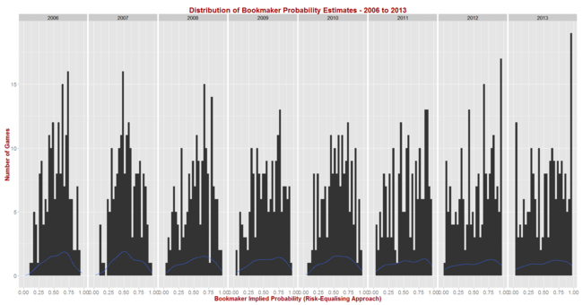
• Calculated the implicit bookmaker probabilities (using the Risk-Equalising approach) for all games in the 2006 to 2013 period
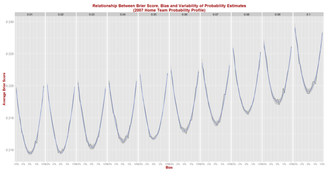
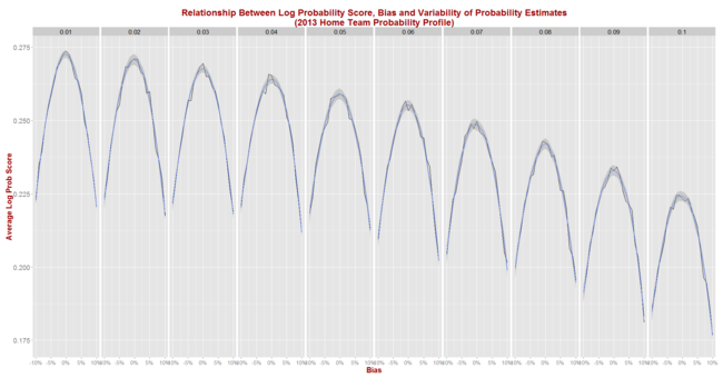
• Assumed that the predictor to be simulated assigns probabilities to games as if making a random selection from a Normal distribution with mean equal to the true probability - as assessed in the step above - plus some bias between -10% and +10% points, and with some standard deviation (sigma) in the range 1% to 10% points. Probability assessments that fall outside the (0.01, 0.99) range are clipped. Better tipsters are those with smaller (in absolute terms) bias and smaller sigma.
• For each of the simulated (bias, sigma) pairs, simulated 1,000 seasons with the true probabilities for every game drawn from the empirical implicit bookmaker probabilities for a specific season.

Before I reveal the results for the first set of simulations let me first report on the season-by-season profile of implicit bookmaker probabilities, based on my TAB Sportsbet data.

The black bars reflect the number of games for which the home team's implicit home team probability fell into the bin-range recorded in the x-axis, and the blue lines map out the smoothed probability density of that same data. These blue lines highlight the similarity in terms of the profile of home team probabilities of the last three seasons. In these three years we've seen quite high numbers of short-priced (ie high probability) home team favourites and few - though not as few as in some other years - long-shot home teams. 

Seasons 2008, 2009 and 2010 saw a more even spread of home team probabilities and fewer extremes of probability at either end, though home team favourites still comfortably outnumbered home team underdogs. Seasons 2006 and 2007 were different again, with 2006 exhibiting some similarities to the 2008 to 2010 period, but with 2007 standing alone as a season with a much larger proportion of contests pitting relatively evenly-matched tips. That characteristic makes prediction more difficult, which we'd expect to be reflected in expected probability scores.

So, with a view to assessing the typical range of Brier Scores under the most diverse sets of conditions, I ran the simulation steps described above once using the home team probability distribution from 2013, and once using the distribution from 2007.

THE BRIER SCORE RESULTS

Here, firstly, are the results for all (bias, sigma) pairs, each simulated for 1,000 seasons that look like 2013.

As we'd expect, the best average Brier Scores are achieved by a tipster with zero bias and the minimum, 1% standard deviation. Such a tipster could expect to achieve an average Brier Score of about 0.167 in seasons like 2013.

For a given standard deviation, the further is the bias from zero the poorer (higher) the expected Brier Score and, for a given bias, the larger the standard deviation the poorer the expected Brier Score as well. So, for example, we can see from the graph that an unbiased tipster with a 5% point standard deviation should expect to record an average Brier Score of about 0.175.

Using Eureqa to fit an equation to the Brier Score data for all 210 simulated (bias, sigma) pairs produces the following approximation:

Expected Brier Score = 0.168 + 0.89 x Bias^2 + 0.87 x Sigma^2

This equation, which explains 98% of the variability in the average Brier Scores across the 210 combinations, suggests that the Brier Score of a tipster is about equally harmed by equivalent changes in percentage point terms in bias and variance (ie sigma squared). Every 1% point change in squared bias or in variance adds about 0.09 to the expected Brier Score.

Next, we simulate Brier Score outcomes for seasons that look like 2007 and obtain the following picture:

The general shape of the relationships shown here are virtually identical to those we saw when using the 2013 data, but the expected Brier Score values are significantly higher.

Now, an unbiased tipster with a 1% point standard deviation can expect to register a Brier Score of about 0.210 per game (up from 0.167), while one with a 5% point standard deviation can expect to return a Brier Score of about 0.212 (up from 0.175).

Eureqa now offers the following equation to explain the results for the 210 (bias, sigma) pairs:

Expected Brier Score = 0.210 + 0.98 x Bias^2 + 0.94 x Sigma^2

This equation explains 99% of the variability in average Brier Scores across the 210 combinations and, when compared with the earlier equation, suggests that: 

• A perfect tipster - that is one with zero bias and zero variance - would achieve a Brier Score of about 0.210 in seasons like 2007 and of 0.168 in seasons like 2013
• Additional bias and variability in a tipster's predictions are punished more in absolute terms in seasons like 2007 than in seasons like 2013. This is evidenced by the larger coefficients on the bias and variance terms in the equation for 2007 compared to those for 2013.

In seasons in which probability estimation is harder - that is, in seasons full of contests pitting evenly-matched teams against one another - Brier Scores will tend to do a better job of differentiating weak from strong predictors. 

THE LPS RESULTS

Though I have performed simulations to determine empirical norms for the LPS metric before, I included this metric in the current round of simulations as well. Electrons are cheap.

Here are the curves for simulations of LPS for the 2013-like seasons.

Eureqa suggests that the relationship between expected LPS, bias and variance is, like that between Brier Score, bias and variance, quadratic in nature, though here the curves are concave rather than convex. We get:

Expected LPS = 0.271 - 4.68 x Bias^2 - 4.71 x Sigma^2

This equation explains 99% of the variability in average LPSs observed across the 210 combinations of bias and sigma.

Finally, simulating using 2007-like seasons gives us this picture.

Again we find that the shape when using the 2007 data is the same as that when using the 2013 data, but the absolute scores are poorer (which here means lower).

Eureqa now offers up this equation:

Expected LPS = 0.127 - 4.17 x Bias^2 - 4.35 x Sigma^2

This equation accounts for 97% of the total variability in average LPS across the 210 simulated pairs of bias and sigma and suggests that expected LPSs in seasons like 2007 are less sensitive to changes in bias and variance than are expected LPSs in seasons like 2013. This is contrary to the result we found for expected Brier Scores, which were more sensitive to changes in bias and variance in seasons like 2007 than in seasons like 2013.

In more challenging predictive environments, therefore, differences in predictive ability as measured by different biases and variances, are likely to result in larger absolute differences in Brier Scores than differences in LPSs.

SUMMARY AND CONCLUSION

We now have some bases on which to make normative judgements about Brier Scores and Log Probability Scores, though these judgements require some knowledge about the underlying distribution of true home team probabilities.

If 2014 is similar to the three seasons that have preceded it then a "good" probability predictor should produce an average Brier Score of about 0.170 to 0.175, and an average LPS of about 0.230 to 0.260. In 2013, the three bookmaker-derived Probability Predictors all finished the season with average LPS' of about 0.260.

[EDIT : It's actually not difficult to derive the following relationship theoretically for a forecaster whose predictions are 0 or 1 with fixed probability and independent of the actual outcome

Expected Brier Score = True Home Probability x (1 - True Home Probability) + Bias^2 + Sigma^2

View fullsize

The proof appears in the image at left.

(Click on the image for a larger version.)

Now the fitted equations for Expected Brier Scores above have coefficients on Bias and Sigma that are less than 1 mostly due, I think, to the effects of probability truncation, which tend to improve (ie lower) Brier Scores for extreme probabilities. There might also be some contribution from the fact that I've modelled the forecasts using a Normal rather than a Binomial distribution.

Deriving a similar equation theoretically rather than empirically for the Expected LPS of a contest is a far more complicated endeavour ...]

Cursory Mention of MAFL in New Scientist (Probably)

At the start of the year, Michael Schmidt, creator of the Eureqa application, mentioned that Justin Mullins from New Scientist was researching for a piece on Eureqa. I dropped an e-mail to Justin, received a polite reply and thought little more of it.

Turns out the final article included this paragraph:

"Today, the algorithm is called Eureqa and has thousands of users all over the world, with people using it for everything from financial forecasting to particle physics. One person even uses it to analyse the statistics of Australian rules football games."

(Various people have cut-and-pasted the full article, for example Transcurve and Kurzweilai, and you can access the original content directly via the New Scientist site if you're willing to create a free subscription.)

I can't be completely certain, but it's more likely than not that the last sentence refers to MAFL.

It'd be nice if the reference was a tad more direct - say with a name or a URL - but then again it'd be preferable if any wider awareness of MAFL's existence came at a time when the Funds were making rather than losing money. So, swings and roundabouts ... 

Adding Some Spline to Your Models

Creating the recent blog on predicting the Grand Final margin based on the difference in the teams' MARS Ratings set me off once again down the path of building simple models to predict game margin.

It usually doesn't take much.

Firstly, here's a simple linear model using MARS Ratings differences that repeats what I did for that recent blog post but uses every game since 1999, not just Grand Finals.

It suggests that you can predict game margins - from the viewpoint of the home team - by completing the following steps:

1. subtract the away team's MARS Rating from the home team's MARS Rating
2. multiply this difference by 0.736
3. add 9.871 to the result you get in 2.

One interesting feature of this model is that it suggests that home ground advantage is worth about 10 points.

The R-squared number that appears on the chart tells you that this model explains 21.1% of the variability is game margins.

You might recall we've found previously that we can do better than this by using the home team's victory probability implied by its head-to-head price.

This model says that you can predict the home team margin by multiplying its implicit probability by 105.4 and then subtracting 48.27. It explains 22.3% of the observed variability in game margins, or a little over 1% more than we can explain with the simple model based on MARS Ratings.

With this model we can obtain another estimate of the home team advantage by forecasting the margin with a home team probability of 50%. That gives an estimate of 4.4 points, which is much smaller than we obtained with the MARS-based model earlier.

(EDIT: On reflection, I should have been clearer about the relative interpretation of this estimate of home ground advantage in comparison to that from the MARS Rating based model above. They're not measuring the same thing.

The earlier estimate of about 10 points is a more natural estimate of home ground advantage. It's an estimate of how many more points a home team can be expected to score than an away team of equal quality based on MARS Rating, since the MARS Rating of a team for a particular game does not include any allowance for whether or not it's playing at home or away.

In comparison, this latest estimate of 4.4 points is a measure of the "unexpected" home ground advantage that has historically accrued to home teams, over-and-above the advantage that's already built into the bookie's probabilities. It's a measure of how many more points home teams have scored than away teams when the bookie has rated both teams as even money chances, taking into account the fact that one of the teams is (possibly) at home.

It's entirely possible that the true home ground advantage is about 10 points and that, historically, the bookie has priced only about 5 or 6 points into the head-to-head prices, leaving the excess of 4.4 that we're seeing. In fact, this is, if memory serves me, consistent with earlier analyses that suggested home teams have been receiving an unwarranted benefit of about 2 points per game on line betting.

Which, again, is why MAFL wagers on home teams.)

Perhaps we can transform the probability variable and explain even more of the variability in game margins.

In another earlier blog we found that the handicap a team received could be explained by using what's called the logit transformation of the bookie's probability, which is ln(Prob/(1-Prob)).

Let's try that.

We do see some improvement in the fit, but it's only another 0.2% to 22.5%. Once again we can estimate home ground advantage by evaluating this model with a probability of 50%. That gives us 4.4 points, the same as we obtained with the previous bookie-probability based model.

A quick model-fitting analysis of the data in Eureqa gives us one more transformation to try: exp(Prob). Here's how that works out:

We explain another 0.1% of the variability with this model as we inch our way to 22.6%. With this model the estimated home-ground advantage is 2.6 points, which is the lowest we've seen so far.

If you look closely at the first model we built using bookie probabilities you'll notice that there seems to be more points above the fitted line than below it for probabilities from somewhere around 60% onwards.

Statistically, there are various ways that we could deal with this, one of which is by using Multivariate Adaptive Regression Splines.

(The algorithm in R - the statistical package that I use for most of my analysis - with which I created my MARS models is called earth since, for legal reasons, it can't be called MARS. There is, however, another R package that also creates MARS models, albeit in a different format. The maintainer of the earth package couldn't resist the temptation not to call the function that converts from one model format to the other mars.to.earth. Nice.)

The benefit that MARS models bring us is the ability to incorporate 'kinks' in the model and to let the data determine how many such kinks to incorporate and where to place them.

Running earth on the bookie probability and margin data gives the following model:

Predicted Margin = 20.7799 + if(Prob > 0.6898155, 162.37738 x (Prob - 0.6898155),0) + if(Prob < 0.6898155, -91.86478 x (0.6898155 - Prob),0)

This is a model with one kink at a probability of around 69%, and it does a slightly better job at explaining the variability in game margins: it gives us an R-squared of 22.7%.

When you overlay it on the actual data, it looks like this.

You can see the model's distinctive kink in the diagram, by virtue of which it seems to do a better job of dissecting the data for games with higher probabilities.

It's hard to keep all of these models based on bookie probability in our head, so let's bring them together by charting their predictions for a range of bookie probabilities.

For probabilities between about 30% and 70%, which approximately equates to prices in the $1.35 to $3.15 range, all four models give roughly the same margin prediction for a given bookie probability. They differ, however, outside that range of probabilities, by up to 10-15 points. Since only about 37% of games have bookie probabilities in this range, none of the models is penalised too heavily for producing errant margin forecasts for these probability values.

So far then, the best model we've produced has used only bookie probability and a MARS modelling approach.

Let's finish by adding the other MARS back into the equation - my MARS Ratings, which bear no resemblance to the MARS algorithm, and just happen to share a name. A bit like John Howard and John Howard.

This gives us the following model:

Predicted Margin = 14.487934 + if(Prob > 0.6898155, 78.090701 x (Prob - 0.6898155),0) + if(Prob < 0.6898155, -75.579198 x (0.6898155 - Prob),0) + if(MARS_Diff < -7.29, 0, 0.399591 x (MARS_Diff + 7.29)

The model described by this equation is kinked with respect to bookie probability in much the same way as the previous model. There's a single kink located at the same probability, though the slope to the left and right of the kink is smaller in this latest model.

There's also a kink for the MARS Rating variable (which I've called MARS_Diff here), but it's a kink of a different kind. For MARS Ratings differences below -7.29 Ratings points - that is, where the home team is rated 7.29 Ratings points or more below the away team - the contribution of the Ratings difference to the predicted margin is 0. Then, for every 1 Rating point increase in the difference above -7.29, the predicted margin goes up by about 0.4 points.

This final model, which I think can still legitimately be called a simple one, has an R-squared of 23.5%. That's a further increase of 0.8%, which can loosely be thought of as the contribution of MARS Ratings to the explanation of game margins over and above that which can be explained by the bookie's probability assessment of the home team's chances.