The Predictability of Game Margins

In a recent blog post I described how the results of games in 2013 have been more predictable than game results from previous seasons in the sense that the final victory margins have been, on average, closer to what you'd have expected them to be based on a reasonably constructed predictive model. In short, teams have this year won by margins closer to what an informed observer, like a Bookmaker, would have expected.
Read More

The Predictability of 2013

Friend of MAFL, Michael, e-mailed me earlier to ask about my claim that 2013 was on track to be the most predictable MAFL season ever, pointing out, quite correctly, that bookmaker favourites have been winning at about the same rate - perhaps even at a slightly higher rate - as they had been at the same time last year.
Read More

Team Scores - Statistical Distribution and Dependence

In the most recent post on the Simulations blog I assumed that Home Team and Away Team scores were independently and Normally distributed (about their conditional means). I'll investigate both these assumptions in this blog.
Read More

Finding Non-Linear Relationships Between AFL Variables : The MINER Package

It's easy enough to determine whether or not one continuous variable has a linear relationship with another, and how strong that relationship is, by calculating the Pearson product-moment correlation coefficient for the two variables. A value near +1 for this coefficient indicates a strong, positive linear relationship between the variables in question, so that high values of one tend to coincide with high values of the other, and vice versa for low values; a value near -1 indicates a strong, negative linear relationship; and a value of 0 indicates a lack of any linear relationship at all. But what if we want to assess more generally if there's a relationship between two variables, linear or otherwise, and we don't know the exact form that this relationship takes? That's the purpose for which the Maximal Information Coefficient (MIC) was created, and recently made available in an R package called MINER.
Read More

Why It Matters Which Team Wins

In conversation - and in interrogation, come to think of it - the key to getting a good answer is often in the framing of the question.

So too in statistical modelling, where one common method for asking a slightly different question of the data is to take the variables you have and transform them.

Consider for example the following results for four binary logits, each built to provide an answer to the question 'Under what circumstances does the team with the higher MARS Rating tend to win?'.
Read More

Adding Some Spline to Your Models

Creating the recent blog on predicting the Grand Final margin based on the difference in the teams' MARS Ratings set me off once again down the path of building simple models to predict game margin.

It usually doesn't take much.

Firstly, here's a simple linear model using MARS Ratings differences that repeats what I did for that recent blog post but uses every game since 1999, not just Grand Finals.

2010 - MARS Ratings vs Score Difference.png

It suggests that you can predict game margins - from the viewpoint of the home team - by completing the following steps:

  1. subtract the away team's MARS Rating from the home team's MARS Rating
  2. multiply this difference by 0.736
  3. add 9.871 to the result you get in 2.

One interesting feature of this model is that it suggests that home ground advantage is worth about 10 points.

The R-squared number that appears on the chart tells you that this model explains 21.1% of the variability is game margins.

You might recall we've found previously that we can do better than this by using the home team's victory probability implied by its head-to-head price.

2010 - Bookie Probability vs Score Difference.png

This model says that you can predict the home team margin by multiplying its implicit probability by 105.4 and then subtracting 48.27. It explains 22.3% of the observed variability in game margins, or a little over 1% more than we can explain with the simple model based on MARS Ratings.

With this model we can obtain another estimate of the home team advantage by forecasting the margin with a home team probability of 50%. That gives an estimate of 4.4 points, which is much smaller than we obtained with the MARS-based model earlier.

(EDIT: On reflection, I should have been clearer about the relative interpretation of this estimate of home ground advantage in comparison to that from the MARS Rating based model above. They're not measuring the same thing.

The earlier estimate of about 10 points is a more natural estimate of home ground advantage. It's an estimate of how many more points a home team can be expected to score than an away team of equal quality based on MARS Rating, since the MARS Rating of a team for a particular game does not include any allowance for whether or not it's playing at home or away.

In comparison, this latest estimate of 4.4 points is a measure of the "unexpected" home ground advantage that has historically accrued to home teams, over-and-above the advantage that's already built into the bookie's probabilities. It's a measure of how many more points home teams have scored than away teams when the bookie has rated both teams as even money chances, taking into account the fact that one of the teams is (possibly) at home.

It's entirely possible that the true home ground advantage is about 10 points and that, historically, the bookie has priced only about 5 or 6 points into the head-to-head prices, leaving the excess of 4.4 that we're seeing. In fact, this is, if memory serves me, consistent with earlier analyses that suggested home teams have been receiving an unwarranted benefit of about 2 points per game on line betting.

Which, again, is why MAFL wagers on home teams.)

Perhaps we can transform the probability variable and explain even more of the variability in game margins.

In another earlier blog we found that the handicap a team received could be explained by using what's called the logit transformation of the bookie's probability, which is ln(Prob/(1-Prob)).

Let's try that.

2010 - Bookie Probability vs Score Difference - Logit Form.png

We do see some improvement in the fit, but it's only another 0.2% to 22.5%. Once again we can estimate home ground advantage by evaluating this model with a probability of 50%. That gives us 4.4 points, the same as we obtained with the previous bookie-probability based model.

A quick model-fitting analysis of the data in Eureqa gives us one more transformation to try: exp(Prob). Here's how that works out:

2010 - Bookie Probability vs Score Difference - Exp Form.png

We explain another 0.1% of the variability with this model as we inch our way to 22.6%. With this model the estimated home-ground advantage is 2.6 points, which is the lowest we've seen so far.

If you look closely at the first model we built using bookie probabilities you'll notice that there seems to be more points above the fitted line than below it for probabilities from somewhere around 60% onwards.

Statistically, there are various ways that we could deal with this, one of which is by using Multivariate Adaptive Regression Splines.

(The algorithm in R - the statistical package that I use for most of my analysis - with which I created my MARS models is called earth since, for legal reasons, it can't be called MARS. There is, however, another R package that also creates MARS models, albeit in a different format. The maintainer of the earth package couldn't resist the temptation not to call the function that converts from one model format to the other mars.to.earth. Nice.)

The benefit that MARS models bring us is the ability to incorporate 'kinks' in the model and to let the data determine how many such kinks to incorporate and where to place them.

Running earth on the bookie probability and margin data gives the following model:

Predicted Margin = 20.7799 + if(Prob > 0.6898155, 162.37738 x (Prob - 0.6898155),0) + if(Prob < 0.6898155, -91.86478 x (0.6898155 - Prob),0)

This is a model with one kink at a probability of around 69%, and it does a slightly better job at explaining the variability in game margins: it gives us an R-squared of 22.7%.

When you overlay it on the actual data, it looks like this.

2010 - Bookie Probability vs Score Difference - MARS.png

You can see the model's distinctive kink in the diagram, by virtue of which it seems to do a better job of dissecting the data for games with higher probabilities.

It's hard to keep all of these models based on bookie probability in our head, so let's bring them together by charting their predictions for a range of bookie probabilities.

2010 - Bookie Probability vs Score Difference - Predictions.png

For probabilities between about 30% and 70%, which approximately equates to prices in the $1.35 to $3.15 range, all four models give roughly the same margin prediction for a given bookie probability. They differ, however, outside that range of probabilities, by up to 10-15 points. Since only about 37% of games have bookie probabilities in this range, none of the models is penalised too heavily for producing errant margin forecasts for these probability values.

So far then, the best model we've produced has used only bookie probability and a MARS modelling approach.

Let's finish by adding the other MARS back into the equation - my MARS Ratings, which bear no resemblance to the MARS algorithm, and just happen to share a name. A bit like John Howard and John Howard.

This gives us the following model:

Predicted Margin = 14.487934 + if(Prob > 0.6898155, 78.090701 x (Prob - 0.6898155),0) + if(Prob < 0.6898155, -75.579198 x (0.6898155 - Prob),0) + if(MARS_Diff < -7.29, 0, 0.399591 x (MARS_Diff + 7.29)

The model described by this equation is kinked with respect to bookie probability in much the same way as the previous model. There's a single kink located at the same probability, though the slope to the left and right of the kink is smaller in this latest model.

There's also a kink for the MARS Rating variable (which I've called MARS_Diff here), but it's a kink of a different kind. For MARS Ratings differences below -7.29 Ratings points - that is, where the home team is rated 7.29 Ratings points or more below the away team - the contribution of the Ratings difference to the predicted margin is 0. Then, for every 1 Rating point increase in the difference above -7.29, the predicted margin goes up by about 0.4 points.

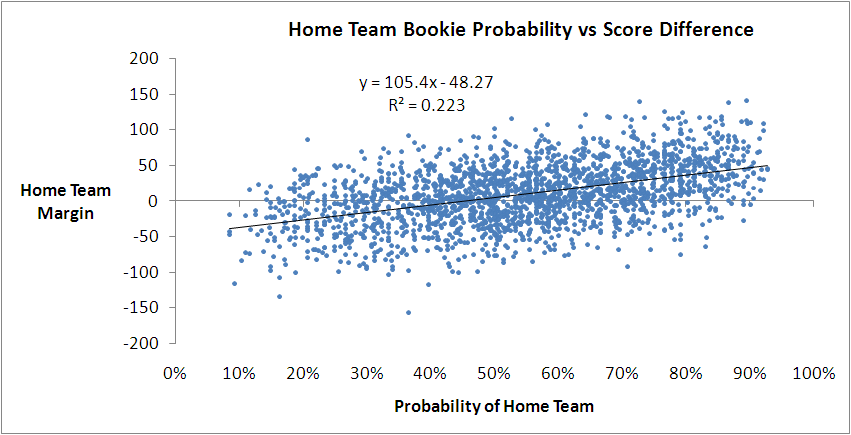
This final model, which I think can still legitimately be called a simple one, has an R-squared of 23.5%. That's a further increase of 0.8%, which can loosely be thought of as the contribution of MARS Ratings to the explanation of game margins over and above that which can be explained by the bookie's probability assessment of the home team's chances.