Set of Games Ratings: A Comparison With VSRS

A few weeks back, Tony introduced the Very Simple Rating System (VSRS). It’s an ELO-style rating system applied to the teams in the AFL, designed so that the difference in the ratings between any pair of teams plus some home ground advantage (HGA) can be interpreted as the expected difference in scores for a game involving those two teams played at a neutral venue. Tony's explored a number of variants of the basic VSRS approach across a number of blogs, but I'll be focussing here on the version he created in that first blog.

Read More

Is That a Good Probability Score - the Brier Score Edition

In recent blogs about the Very Simple Ratings System (VSRS) I've been using as my Probability Score metric the Brier Score, which assigns scores to probability estimates on the following basis:

Brier Score = (Actual Result - Probability Assigned to Actual Result)^2

For the purposes of calculating this score the Actual Result is treated as (0,1) variable, taking on a value of 1 if the team in question wins, and a value of zero if that team, instead, loses. Lower values of the Brier Score, which can be achieved by attaching large probabilities to teams that win or, equivalently, small probabilities to teams that lose, reflect better probability estimates.

Elsewhere in MAFL I've most commonly used, rather than the Brier Score, a variant of the Log Probability Score (LPS) in which a probability assessment is scored using the following equation:

Log Probability Score = 1 + logbase2(Probability Associated with Winning team)

In contrast with the Brier Score, higher log probabilities are associated with better probability estimates.

Both the Brier Score and the Log Probability Score metrics are what are called Proper Scoring Rules, and my preference for the LPS has been largely a matter of taste rather than of empirical evidence of superior efficacy.

Because the LPS has been MAFL's probability score of choice for so long, however, I have previously written a blog about empirically assessing the relative merits of a predictor's season-average LPS result in the context of the profile of pre-game probabilities that prevailed in the season under review. Such context is important because the average LPS that a well-calibrated predictor can be expected to achieve depends on the proportion of evenly-matched and highly-mismatched games in that season. (For the maths on this please refer to that earlier blog.)

WHAT'S A GOOD BRIER SCORE?

What I've not done previously is provide similar, normative data about the Brier Score. That's what this blog will address.

Adopting a methodology similar to that used in the earlier blog establishing the LPS norms, for this blog I've: 

  • Calculated the implicit bookmaker probabilities (using the Risk-Equalising approach) for all games in the 2006 to 2013 period
  • Assumed that the predictor to be simulated assigns probabilities to games as if making a random selection from a Normal distribution with mean equal to the true probability - as assessed in the step above - plus some bias between -10% and +10% points, and with some standard deviation (sigma) in the range 1% to 10% points. Probability assessments that fall outside the (0.01, 0.99) range are clipped. Better tipsters are those with smaller (in absolute terms) bias and smaller sigma.
  • For each of the simulated (bias, sigma) pairs, simulated 1,000 seasons with the true probabilities for every game drawn from the empirical implicit bookmaker probabilities for a specific season.

Before I reveal the results for the first set of simulations let me first report on the season-by-season profile of implicit bookmaker probabilities, based on my TAB Sportsbet data.

The black bars reflect the number of games for which the home team's implicit home team probability fell into the bin-range recorded in the x-axis, and the blue lines map out the smoothed probability density of that same data. These blue lines highlight the similarity in terms of the profile of home team probabilities of the last three seasons. In these three years we've seen quite high numbers of short-priced (ie high probability) home team favourites and few - though not as few as in some other years - long-shot home teams. 

Seasons 2008, 2009 and 2010 saw a more even spread of home team probabilities and fewer extremes of probability at either end, though home team favourites still comfortably outnumbered home team underdogs. Seasons 2006 and 2007 were different again, with 2006 exhibiting some similarities to the 2008 to 2010 period, but with 2007 standing alone as a season with a much larger proportion of contests pitting relatively evenly-matched tips. That characteristic makes prediction more difficult, which we'd expect to be reflected in expected probability scores.

So, with a view to assessing the typical range of Brier Scores under the most diverse sets of conditions, I ran the simulation steps described above once using the home team probability distribution from 2013, and once using the distribution from 2007.

THE BRIER SCORE RESULTS

Here, firstly, are the results for all (bias, sigma) pairs, each simulated for 1,000 seasons that look like 2013.

As we'd expect, the best average Brier Scores are achieved by a tipster with zero bias and the minimum, 1% standard deviation. Such a tipster could expect to achieve an average Brier Score of about 0.167 in seasons like 2013.

For a given standard deviation, the further is the bias from zero the poorer (higher) the expected Brier Score and, for a given bias, the larger the standard deviation the poorer the expected Brier Score as well. So, for example, we can see from the graph that an unbiased tipster with a 5% point standard deviation should expect to record an average Brier Score of about 0.175.

Using Eureqa to fit an equation to the Brier Score data for all 210 simulated (bias, sigma) pairs produces the following approximation:

Expected Brier Score = 0.168 + 0.89 x Bias^2 + 0.87 x Sigma^2

This equation, which explains 98% of the variability in the average Brier Scores across the 210 combinations, suggests that the Brier Score of a tipster is about equally harmed by equivalent changes in percentage point terms in bias and variance (ie sigma squared). Every 1% point change in squared bias or in variance adds about 0.09 to the expected Brier Score.

Next, we simulate Brier Score outcomes for seasons that look like 2007 and obtain the following picture:

The general shape of the relationships shown here are virtually identical to those we saw when using the 2013 data, but the expected Brier Score values are significantly higher.

Now, an unbiased tipster with a 1% point standard deviation can expect to register a Brier Score of about 0.210 per game (up from 0.167), while one with a 5% point standard deviation can expect to return a Brier Score of about 0.212 (up from 0.175).

Eureqa now offers the following equation to explain the results for the 210 (bias, sigma) pairs:

Expected Brier Score = 0.210 + 0.98 x Bias^2 + 0.94 x Sigma^2

This equation explains 99% of the variability in average Brier Scores across the 210 combinations and, when compared with the earlier equation, suggests that: 

  • A perfect tipster - that is one with zero bias and zero variance - would achieve a Brier Score of about 0.210 in seasons like 2007 and of 0.168 in seasons like 2013
  • Additional bias and variability in a tipster's predictions are punished more in absolute terms in seasons like 2007 than in seasons like 2013. This is evidenced by the larger coefficients on the bias and variance terms in the equation for 2007 compared to those for 2013.

In seasons in which probability estimation is harder - that is, in seasons full of contests pitting evenly-matched teams against one another - Brier Scores will tend to do a better job of differentiating weak from strong predictors. 

THE LPS RESULTS

Though I have performed simulations to determine empirical norms for the LPS metric before, I included this metric in the current round of simulations as well. Electrons are cheap.

Here are the curves for simulations of LPS for the 2013-like seasons.

Eureqa suggests that the relationship between expected LPS, bias and variance is, like that between Brier Score, bias and variance, quadratic in nature, though here the curves are concave rather than convex. We get:

Expected LPS = 0.271 - 4.68 x Bias^2 - 4.71 x Sigma^2

This equation explains 99% of the variability in average LPSs observed across the 210 combinations of bias and sigma.

Finally, simulating using 2007-like seasons gives us this picture.

Again we find that the shape when using the 2007 data is the same as that when using the 2013 data, but the absolute scores are poorer (which here means lower).

Eureqa now offers up this equation:

Expected LPS = 0.127 - 4.17 x Bias^2 - 4.35 x Sigma^2

This equation accounts for 97% of the total variability in average LPS across the 210 simulated pairs of bias and sigma and suggests that expected LPSs in seasons like 2007 are less sensitive to changes in bias and variance than are expected LPSs in seasons like 2013. This is contrary to the result we found for expected Brier Scores, which were more sensitive to changes in bias and variance in seasons like 2007 than in seasons like 2013.

In more challenging predictive environments, therefore, differences in predictive ability as measured by different biases and variances, are likely to result in larger absolute differences in Brier Scores than differences in LPSs.

SUMMARY AND CONCLUSION

We now have some bases on which to make normative judgements about Brier Scores and Log Probability Scores, though these judgements require some knowledge about the underlying distribution of true home team probabilities.

If 2014 is similar to the three seasons that have preceded it then a "good" probability predictor should produce an average Brier Score of about 0.170 to 0.175, and an average LPS of about 0.230 to 0.260. In 2013, the three bookmaker-derived Probability Predictors all finished the season with average LPS' of about 0.260.

[EDIT : It's actually not difficult to derive the following relationship theoretically for a forecaster whose predictions are 0 or 1 with fixed probability and independent of the actual outcome

Expected Brier Score = True Home Probability x (1 - True Home Probability) + Bias^2 + Sigma^2

The proof appears in the image at left.

(Click on the image for a larger version.)

Now the fitted equations for Expected Brier Scores above have coefficients on Bias and Sigma that are less than 1 mostly due, I think, to the effects of probability truncation, which tend to improve (ie lower) Brier Scores for extreme probabilities. There might also be some contribution from the fact that I've modelled the forecasts using a Normal rather than a Binomial distribution.

Deriving a similar equation theoretically rather than empirically for the Expected LPS of a contest is a far more complicated endeavour ...]

Estimating Team-and-Venue Specific Home Ground Advantage Using the VSRS

In the Very Simple Rating System as I've described it so far, a single parameter, HGA, is used to adjust the expected game margin to account for the well-documented advantages of playing at home. We found that, depending on the timeframe we consider and the performance metric that we chose to optimise, the estimated size of this advantage varied generally in the 6 to 8-point range.
Read More

Optimising the Very Simple Rating System (VSRS)

In the previous blog, introducing the VSRS, I provided optimal values for the tuning parameters of that System, optimal in the sense that they minimised either the mean absolute or the mean squared error across the period 1999 to 2013
Read More

A Very Simple Team Ratings System

Just this week, 23 year-old chess phenom Magnus Carlsen wrested the title of World Champion from Vishwathan Anand, in so doing lifting his Rating to a stratospheric 2,870. Chess, like MAFL, uses an an ELO-style Rating System to assess and update the strength of its players.
Read More

Estimating Home Ground Advantage by Venue

In the previous blog I fitted models to the game margins of each team separately, seeking to explain the margin in any game in terms of the Venue at which the game was played and three "Excess" variables summarising from the designated home team's perspective its relative Venue Experience, MARS Rating and recent form.
Read More

What's More Important: Who You Play or Where You Play Them?

The benefits of playing at home have been extensively investigated both here on MAFL for Australian Rules football and more generally within the sports prediction community for this and other sports. Put simply, teams that play at home win more often and score more points than you'd otherwise expect them to after adjusting for the quality of the opponents they face.
Read More

Revisiting Home Ground Advantage

This week I've been part of a Twitter conversation about Home Ground Advantage in the AFL, a trending topic because of the shift from Football Park to Adelaide Oval for the home games of Adelaide and Port Adelaide in the 2014 season.
Read More

MARS Rating Changes and Scoring Percentages: 1897-2013

The idea for this blog sprang from some correspondence with Friend of MAFL, Michael, so let me start by thanking him for being the inspiration. Michael was interested in exploring the relationship between team performances and the resulting change in their MARS Ratings across a season, which I'll explore here by charting, for each team and every season, the for-and-against percentage they achieved in all games including Finals, and the change in their MARS Rating per game during that same season.
Read More

Another View of All-Time AFL Team MARS Ratings Post the 2013 Season

Recently I'd been noticing some traffic to the site from the Big Footy website where the Forum members had been discussing the relative strengths of Bulldogs teams across VFL/AFL history. That, coupled with my continuing desire to become more proficient in the ggplot2 R package of Hadley Wickham, dragged me out of my off-season blog malaise to perform the analyses underpinning this current posting.
Read More

Building Your Own Team Rating System

Just before the 2nd Round of 2008 I created MAFL's Team Ratings System, MARS, never suspecting that I'd still be writing about it 5 years later. At the time, I described MARS in the newsletter for that week in a document still available from the Newsletters 2005-2008 section section of this website (it's linked under the "MAFL The Early Years" menu item in the navigation bar on the right of screen). Since then, MARS, as much to my surprise as I think to anyone's, has been a key input to the Line Funds that have operated in each of the ensuing years.
Read More

How Good Are Hawthorn, How Poor GWS?

Without the benefit of emotional and chronological distance it's often difficult to rate the historical merit of recent sporting performances. MAFL's MARS Ratings, whilst by no means the definitive measure of a team's worth, provides one, objective basis on which to assess the teams that ran around in 2013.
Read More

Really Simple Margin Predictors : 2013 Review

MAFL's two new Margin Predictors for 2013, RSMP_Simple and RSMP_Weighted, finished the season ranked 1 and 2 with mean absolute prediction errors (MAPEs) under 27 points per game. Historically, I've considered any Predictor I've created as doing exceptionally well if it's achieved a MAPE of 30 points per game or less in post-sample, live competition. An MAPE of 27 is in a whole other league.
Read More

To Win A Grand Final You Must First Lead

History suggests that, as the higher-Rated "Home" team, Hawthorn must lead early and lead well if it is to be confident of success in Saturday's Grand Final, and not assume that its superior Rating will allow it to come back from any substantial deficit.
Read More

The Relative Importance of Class and Form in AFL

Today's blog is motivated by a number of things, the first of which is alluded to in the title: the quantitative exploration of the contributions that teams' underlying class or skill plays in their success in a given game relative to their more recent, more ephemeral form. Is, for example, a top-rated team that's been a little out of form recently more or less likely to beat a less-credentialled team that's been in exceptional form?
Read More

Bookmaker Overround: Relating Team Overround to Victory Probability

In the previous blog I described a general framework for thinking about Bookmaker overround.

There I discussed, in the context of the two-outcome case, the choice of a functional form to describe a team's overround in terms of its true probability as assessed by the Bookmaker. As one very simple example I suggested oi = (1-pi), which we could use to model a Bookmaker who embeds overround in the price of any team by setting it to 1 minus the team's assessed probability of victory. 

Whilst we could choose just about any function, including the one I've just described, for the purpose of modelling Bookmaker overround, choices that fit empirical reality are actually, I now realise, quite circumscribed. This is because of the observable fact that the total overround in any head-to-head market, T, appears to be constant, or close to it, in every game regardless of the market prices, and hence the underlying true probability assessments, of the teams involved. In other words, the total overround in the head-to-head market when 1st plays last is about the same as when 1st plays 2nd.

So, how does this constrain our choice of functional form? Well we know that T is defined as 1/m1 + 1/m2 - 1, where mi is that market price for team i, and that mi = 1/(pi(1+oi)), from which we can determine that: 

  • T = p1(o1 - o2) + o2

If T is to remain constant across the full range of values of p1 then, we need the derivative with respect to p1 of the RHS of this equation to be zero for all values of p1. This implies that the functions chosen for o1 and o2 must satisfy the following equality: 

  • p1(o1' - o2') + o2' = o2 - o1 (where the dash signifies a derivative with respect to p1).

I doubt that many functional forms o1 and o2 (both of which we're assuming are functions of p1, by the way) exist that will satisfy this equation for all values of p1, especially if we also impose the seemingly reasonable constraint that o1 and o2 be of equivalent form, albeit it that o1 might be expressed in terms of p1 and o2 in terms of (1-p1), which we can think of as p2.

Two forms that do satisfy the equation, the proof of which I'll leave as an exercise for any interested reader to check, are: 

  • The Overround-Equalising approach : o1 = o2 = k, a constant, and
  • The Risk-Equalising approach : o1 = e/p1; o2 = e/(1-p1), with e a constant 

There may be another functional form that satisfies the equality above, but I can't find it. (There's a rigorous non-existence proof for you.) Certainly oi = 1 - pi, which was put forward earlier, doesn't satisfy it, and I can postulate a bunch of other plausible functional forms that similarly fail. What you find when you use these forms is that total overround changes with the value of p1.

So, if we want to choose functions for o1 and o2 that produce results consistent with the observed reality that total overround remains constant across all values of the assessed true probability of the two teams it seems that we've only three options (maybe four): 

  1. Assume that the Bookmaker follows the Overround-Equalising approach
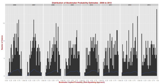
  2. Assume that the Bookmaker follows the Risk-Equalising approach
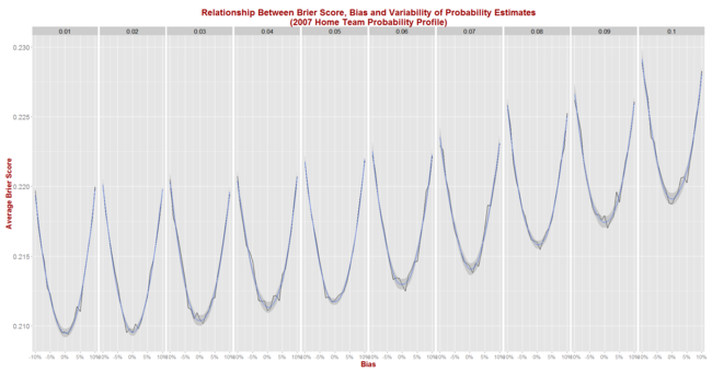
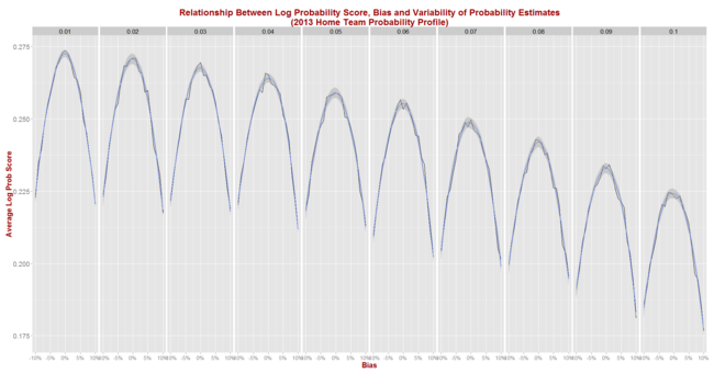
  3. Assume that the Bookmaker chooses one team, say the favourite or the home team, and establishes its overround using a pre-determined function relating its overround to its assessed victory probability. He then sets a price for the other team that delivers the total overround he is targetting. This is effectively the path I followed in this earlier blog where I described what's come to be called the Log Probability Score Optimising (LPSO) approach.

A fourth, largely unmodellable option would be that he simultaneously sets the market prices of both teams so that they together produce a market with the desired total overround while accounting for his assessment of the two team's victory probabilities so that a wager on either team has negative expectation. He does this, we'd assume, without employing a pre-determined functional form for the relationship between overround and probability for either team. 

If these truly are the only logical options available to the Bookmaker then MAFL, it turns out, is already covering the complete range since we track the performance of a Predictor that models its probability assessments by following an Overround-Equalising approach, of another Predictor that does the same using a Risk-Equalising approach, and of a third (Bookie_LPSO) that pursues a strategy consistent with the third option above. That's serendipitously neat and tidy.

The only area for future investigation would be then to seek a solution superior to LPSO for the third approach described above. Here we could use any of the functional forms I listed in the previously blog, but could only apply them to the determination of the overround for one of the teams - say the home team or the favourite - with the price and hence overround for the remaining team determined by the need to produce a market with some pre-specified total overround.

That's enough for today though ...

Bookmaker Overround: A General Framework

Previously I've developed the notion of taking a Bookmaker's prices in the head-to-head market and using them to infer his opinion about the true victory probabilities of the competing teams by adopting an Overround-Equalising or a Risk-Equalising approach. In this blog I'll be summarising and generalising these approaches.
Read More

Team Ratings, Bookmaker Prices and the Recent Predictability of Finals

Last weekend saw three of four underdogs prevail in the first week of the Finals. Based on the data I have, you'd need to go back to 2006 to find a more surprising Week 1 of the Finals and, as highlighted in the previous blog, no matter how far you went back you wouldn't find a bigger upset than Port Adelaide's defeat of the Pies.
Read More