A Very Simple Team Ratings System
/Just this week, 23 year-old chess phenom Magnus Carlsen wrested the title of World Champion from Vishwathan Anand, in so doing lifting his Rating to a stratospheric 2,870. Chess, like MAFL, uses an an ELO-style Rating System to assess and update the strength of its players.
ELO-style Systems reward players - or, in MAFL's case, teams - differentially for the results they achieve based on the relative strength of the opponent they faced. So, for example, a weak player defeating a stronger player benefits more in terms of increased Rating than does a stronger player in defeating a weaker one.
Recently, I published a blog about ELO-style Systems and how you might go about constructing your own Team Rating System using this approach. MARS, the System used on MAFL, is a relatively complex version of such a Rating System, mainly because of the elaborate formulae it uses to calculate an actual result based on a game margin and to calculate the expected result given the competing teams' Ratings.
There is though, I now realise, a much simpler (or a Very Simple, to give it the first part of its proposed name) approach that we might employ to generate an ELO-style Team Ratings.
THE EQUATIONS
Let me start by defining the basic equations for a Very Simple Rating System (VSRS).
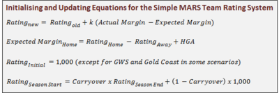
The first equation, which is written from the viewpoint of the Home team, is standard for something ELOvian and states that the home team's new Rating after a game is merely equal to what it was pre-game plus some multiple of the difference between the result it achieved and the result that might have been expected. (The Away team's Rating changes by the same amount, but in the opposite direction.)
In this equation, the Actual Margin is defined in the usual way, as the points scored by the Home team less the points conceded by them. What we need is some reasonable basis on which to determine an Expected Margin for the Home team, and what simpler way can be imagined to do this than to set it equal to the difference between the pre-game Ratings of the Home and the Away team, adjusted for Home Ground Advantage?
So, for example, if a team Rated 1,020 meets a team Rated 1,000 at home, we expect them to win by 20 points plus whatever we assume the Home Ground Advantage to be. This approach provides for a very intuitive definition of a team's Ratings relative to its opponent's: it's how many points better or worse than them they are.
The next equation tells us that all teams begin with a Rating of 1,000 (except, maybe, GWS and the Gold Coast, which I'll discuss later), while the final equation lays down the basis on which teams' Ratings will be carried over from one season to the next.
In total, this basic System requires us to define three parameters:
- k, the multiple by which to convert the difference between Actual and Expected Margins into changes in Ratings
- HGA, the average advantage, in points, assumed to accrue to a home team, which we'll assume to be the same for each team and every venue (although we could do otherwise, though perhaps not for a System labelled Very Simple), and
- Carryover, the proportion of a team's Rating that carries over from one season to the next.
CREATING RATINGS
For this blog I'll be creating Very Simple Team Ratings for the period from the start of the 1999 season to the end of the 2013 season.
For an initial version of this System I'm going to fix the value of the Carryover parameter and choose optimal values for the two parameters, k and HGA, based on some metric. Actually, here, and throughout this blog, I'm going to use two metrics, both of which follow naturally from the second equation above, which posits that the predicted margin for a game is equal to the difference in the team Ratings, adjusted for Home Ground Advantage.
Specifically, I'm going to choose k and HGA (for a given value of Carryover) to minimise:
- The Sum of Squared Errors between the Actual and Expected game margins, summed across all the games from 1999 to 2013
- The Sum of Absolute Errors between the Actual and Expected game margins, also summed across all the games from 1999 to 2013
So, imagine that we used some trial values of k and HGA to determine the Ratings of every team before and after every game in the period 1999 to 2013, and then used those Ratings along with the actual results of every game to calculate the prediction error for each game as
Error = Actual Margin - (RatingHome - RatingAway + HGA)
We then calculate the sum of the absolute value of these errors, in one case, and the sum of the square of these errors in another, and we repeat this whole process for a constrained range of values for k and HGA to find optima, one for each error metric.
Using the Solver function in Excel for this purpose we obtain the results shown in the following table.
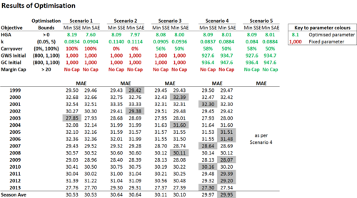
The leftmost columns show the calculated optima when Carryover is fixed at 100%, so that teams enter the first game of a new season with a Rating equivalent to that with which they exited the old one. In this scenario, the optimal Home Ground Advantage if we minimise the squared errors between actual and expected game margins is about 8.2 points and the optimal value of k is about 0.0834.
These values of k and HGA imply that we should update the Rating of the Home team by taking a little over 8% of the difference between the game margin it achieved and the game margin we expected, adjusting for an assumed 8-point Home Ground Advantage.
So, for example, if a Home team Rated 1,010 defeated a team Rated 990 by 25 points, the adjustment to its Rating would be 0.0834 x (25 - (1,010 - 990 + 8.19)), which is -0.266. The Home team's Rating declines in this example because, with the roughly 8 point HGA and its pre-game 20 point Rating superiority, the Home team was expected to win by about 28 points but actually won by only 25 points. In this example, the Away team's Rating would increase by the same amount.
This first, very simple Very Simple system is already quite good at predicting game margins, recording about a 30.5 mean squared (MSE) if we calculate a season-average of the season-by-season results, and recording a 27.7 points per game MAE for season 2013 considered alone, a performance good enough for 7th place on the MAFL Leaderboard last season.
If we maintain this same 100% Carryover but instead minimise mean absolute prediction error (MAE), the optimal value of HGA drops a little to 7.6, and of k rises to 0.904. These values make for a System that, produces a slightly higher MAE per game (but, though not shown here, a smaller MSE since that's what it's minimising).
In the next block of the table we fix Carryover at 0% so that teams enter each year anew with a 1,000 Rating. This results in poorer Team Ratings, at least if we consider MAE per game to be our performance metric. Optimising HGA and k under the assumption of a 0% Carryover results in a System with about an 0.1 points per game poorer MAE across the 15 seasons and about 1.5 to 1.6 points per game poorer MAE for season 2013.
OPTIMISING CARRYOVER
For the third block in the table above, which I've labelled Scenario 3 to preserve the MAFL tradition of prosaicness in nomenclature, I've made Carryover a free variable constrained only to the (0,1) range, and thereby identified a Rating System that is superior by about 0.4 points per game. The optimal values of k and HGA change by just a little from the values we had previously, to about 0.09 for k and 8 for HGA, while the optimal Carryover is either 56% if we're seeking to minimise MSE, or 50% if we're seeking to minimise MAE.
RATING NEW TEAMS
Long-term MAFL readers might remember the deliberations about the appropriate initial MARS Ratings to use for Gold Coast and GWS when they entered the competition. In the end, Gold Coast were MARS Rated 1,000 and GWS 900, in the latter case with at least some (at the time) recent empirical data to factor into the decision, albeit for a different team from another State.
With the benefit of hindsight we can now find optimum Ratings for these two teams, setting them to values which assist us in out quest to minimise the differences between Actual and Expected game margins, which I do for the first time in Scenario 4. Depending on whether we choose to minimise squared or absolute errors, GWS' optimal initial Rating is either 928 or 935, and Gold Coast's is either 936 or 948. Those results suggest that when GWS started they were about 65 to 70 points inferior to an average team, and when Gold Coast started they were about 50 to 65 points inferior.
This new, optimised Very Simple Rating System (VSRS) gives margin predictions with an MAE of just under 30 points per game across the 15 seasons and with an MAE of 27.39 points per game for 2013, a performance still only good enough for 7th on the MAFL Leaderboard but now just 0.04 points per game behind the 6th-placed Bookie_3.
CAPPING MARGINS
MARS, in an effort to limit the impact on team Ratings of blowout victories, caps the victory margins that it recognises for the purpose of updating team Ratings. If a team wins (or loses) by more than 78 points, an adjusted victory margin of 78 points is used to calculate new Ratings in place of the actual margin.
When I offer the VSRS the opportunity to select an optimal margin cap, it assesses the optimal margin cap as being no cap at all. In other words, every point scored or conceded by either team is assessed as being relevant for optimally updating their Ratings, even in blowout games. Accordingly, the results shown for Scenario 5 in the table above are the same as those shown for Scenario 4.
SUMMARISING THE VERY SIMPLE RATING SYSTEM (VSRS)
So, we finish with an optimised VSRS as follows:
- RatingHome_new = RatingHome_old + 0.0884 x (Actual Margin - Expected Margin)
- Expected MarginHome = RatingHome - RatingAway + 8.01
- Actual MarginHome = Points ScoredHome - Points ScoredAway
- RatingAway_new = RatingAway_old - (RatingHome_new - RatingHome_old)
- Initial Ratings (as at Round 1 of 1999) = 1,000 for all teams except GWS and Gold Coast
- Intital Rating for Gold Coast = 947.6
- Intital Rating for GWS = 934.7
- RatingNew_Season = 0.5 x RatingPrevious_Season + 500
This System has a season-average MAE across the 1999 to 2013 seasons of 29.95 points per game, just less than the magic figure of 30.
AN EMPIRICAL EXAMPLE: THE END OF THE 2013 SEASON

If we apply this System to the seasons from 1999 to 2013 we wind up with the Ratings shown in the table at left as the position at the end of last season.
There we see that the Hawks are Rated about 6.7 points better than the Cats (meaning that we'd predict a 14.7 points win by the Hawks if they're playing the Cats at home, and a 1.3 point loss if they're facing them away), and that the Hawks are Rated over 95 points better than the Giants.
On the righthand side of the table are the standard MARS Ratings as at the end of season 2013, which are very similar to the VSRS Ratings both in terms of team Ratings (the correlation is over +0.98) and team Rankings.
The only differences in Ranking of more than a single spot are for the Lions, ranked 11th by VSRS and 13th by MARS; the Saints, ranked 12th by VSRS and 14th by MARS; Essendon, ranked 13th by VSRS and 10th by MARS; and the Eagles, ranked 14th by VSRS and 12th by MARS. Five other teams have Rankings that differ by a single spot, and nine more have the same Ranking under both Systems.
Next season I'll probably track the performance of VSRS, or of a System built using the same principles, alongside the performances of MARS, Colley, Massey and ODM.
Regardless, interested readers now have a basis on which to create and track their own team ratings.