Valuing Draft Picks Based on Career AFL Ratings Output
/INTRODUCTION
With all the attention paid to the men’s National Draft for the AFL and the commentary about the value of getting early picks, it seems only natural to build a model that estimates the relative value of each pick.
“Value”, of course, is a tricky term. It’s easy to imagine a range of metrics that might be used to measure it, from things as simple as career length to career wins right up to more complex metrics that seek to measure a player’s individual impact on results.
Whilst recognising that AFL Player Ratings are not perfect, they do, at least correlate highly with other metrics such as Coaches Votes and Brownlow Votes - although they too are imperfect - and they are designed to produce a measure of each player’s impact on their team’s performance.
All of which is a slightly hand-wavy way of saying that I’ve chosen to use AFL Player Rating as the value metric for this analysis and, knowing that these Ratings systematically differ by position, have investigated how the results are affected if position is taken into account.
To get in one more caveat before revelaing the results I should also point out that what we’re measuring is revealed not latent value. It could well be that Player X would have had a very different career, AFL Rating Point-wise, had he played for Team A rather than Team B, but that’s something impossible to account for unless and until someone gets access to one of the other multiverses in which Patrick Dangerfield plays his entire career at North Melbourne.
Lastly, I should highlight that I don’t expect my results to match those in the original AFL DVI or the DVI after the 2025 changes because:
the original DVIs were based on player salary data from 2000-2014
the changes made in 2025 reflect a policy objective that involves reducing the points attached to later selections to make it harder for clubs to accumulate late picks and use them to match bids on highly rated players
In passing, I should note that I’ve never been able to understand why the original DVI curve, which appears on page 6 of that PDF, shows a “fitted” curve so apparently not fitted to the data. In the image at right I’ve added a new fit that seems to better match the data.
It drops away far more sharply for early picks and plateaus much more for later picks.
Coincidentally, the 2025 changes produce a curve that better fits the raw data in the 2015 analysis although it still doesn’t fall away fast enough in the early picks.
To summarise, the AFL DVIs are based on salary - essentially equating value with market prices - with an overlay of policy. My DVIs will be based solely on AFL Player Ratings.
METHODOLOGY AND DATA
To be specific, I’ve used AFL Player Rating Points as the measure of value at the game level, so a career is valued at the sum of its ratings across all games, including any played after changing clubs. Career data suffers from what’s called censoring - right censoring in this case - because many players in the data have not yet retired. To estimate the remaining career value for these players I need two numbers for every potential future game: the chance the player gets there, and their expected AFL Player rating if they do. Multiplying those numbers and adding up over the extra career gives the pick’s expected future value.
In presenting the results I’ve also chosen to focus on the seasons from 2012 to 2026, which are those for which there is AFL Rating Data on the AFL site. I have, however, included any player who debuted in season 2000 or later and who has Rating Data in the 2012 to 2026 window. That amounts to 1,557 linked National Draft debutants from 2000 to 2026, comprising 874 who debuted from 2012 onward and 683 who debuted earlier.
AFL Tables supplied appearances and career game numbers, while the AFL match feed supplied 100,987 observed individual match ratings from 2012 onward. Pre-2012 debutants contributed career-length information and, where available, ratings recorded from 2012 at their actual career game numbers.
Historical draft records and player profiles were reconciled to identify each player’s first entry, excluding rookie entrants subsequently selected in the National Draft. Historical name changes, ambiguous matches and unrecorded earlier entries remain sources of error. Sources include AFL Tables, Draftguru, Footywire and the fitzRoy package.
One very important adjustment I need to make is for players who are drafted but who never make their senior debut. The table below provides a summary of how often this occurs for players drafted in particular Pick number bins.
The raw data to this table informs a logistic debut probability model as shown at right, where p is Pick number.
Without this adjustment we’d risk overstating the relative value of any cohort that produces a larger number of players who never debut. Here we can see that this particularly applies to higher Pick numbers.
ANALYSES
Valuing National Draft Picks
Suppose the first player taken in the men’s National Draft debuts and goes on to produce 100 units of career value using AFL Player Ratings as the metric What would we expect from a player taken at Pick 20 who also makes it to senior football? What about Pick 40, and where does the difference comes from.
For this analysis we fit models that estimate two quantities for a player taken at pick P:
Expected Match-Rating: the rating they are expected to earn in career game g, and
Estimated Career Length: the probability that game g will be a player’s last, given that they reach it
A career-value curve comes from combining those two estimates.
Expected Match-Rating
For this model we fit a flexible functional form as described below.
The fitted values for this equation are as follows:
Estimated Career Length:
For this model we fit a flexible logistic functional form as described below.
A player’s career was deemed over if he:
had a Footywire past-player record with a recorded last-playing year, and appeared on no current list
did not appear on any current Footywire club list and had missed at least two completed seasons
Players whose status was unresolved by these rules were treated as active.
The fitted values for this equation are as follows:
These two models, combined with the earlier debut probability model, are then used to produce a pick-relative value curve as follows:
Note that only 42 players in the post-debut modelling sample had reached game 300 by the end of the observation period. To account for games after this milestone I hold each Pick numbers exit risk and expected match rating constant at the value for game 300 and sum the remaining tail analytically. That tail contributes about 12.5% of Pick 1’s expected career value and 9.0% of Pick 20’s, including the adjustment for non-debutants. Moving the tail boundary to game 250 or 350 changes Pick 20’s relative value to 54.4 or 56.0, respectively, compared with 55.6 under the 300-game assumption. The approximate confidence intervals account for repeated observations on the same player, uncertainty in estimated debut probability, and uncertainty in the Pick 1 denominator, and for the fact that some of the same players contribute to more than one model and might therefore have correlated errors.
Using this equation the model values Pick 1 at 2,883 career Rating Points, and Pick 2 at about 2,651, or 92% of the Pick 1 value. At Pick 20 the estimate falls to 1,602 or about 56%.
Figure 1. Expected aggregate career AFL Rating Points relative to pick 1, conditional on a senior debut.
An approximate equation for the curve where p is the pick number and V the relative value is:
V(p) = 100 - 8.33821 x ln(p) - 2.23548 x [ln(p)]^2
The table below provides specific values for specific pick numbers and gives an indication of the range of possible values and the number of players for whom full data is available. There are 27 observed debutants at Pick 1 and just one at Pick 80. The number of debutants at higher pick numbers tend to be smaller: because some drafts don’t get to the point where those pick numbers are used.
Fitting a constrained curve to the outputs allows the results for nearby pick numbers to inform the estimate for picks with little observed data.
Table 1. Estimated career value at selected National Draft picks.
Why these functional forms?
There is no obviously correct functional form for either model but the chosen form for the expected match rating model has the following advantages:
Taking the log of Pick number gives more resolution near the top of the draft. A one-place move from Pick 1 to Pick 2 changes ln(p) by 0.693, while moving from 40 to 41 changes it by only 0.025. That provides for greater separation of the early picks.
Using a spline provides for changes in the shape of the curve across different parts of the career. Imposing a linear game number effect would force the same change in expected rating in moving from from game 5 to game 15 as from game 205 to game 215. As with using the log of Pick number, using the log of game number provides for greater separation during the early career. The spline then lets the model reflect development as a plateau or a decline. The knots at games 10, 60 and 150 are modelling choices that provide flexibility across early, established and long careers.
The interaction term involving Pick number and career game accounts for the possibility that different Pick numbers might have different trajectories. As included in the model it allows the expected rating gap between two Pick numbers to widen or narrow as the career game count increases.
The chosen form for the career exit model has the following advantages:
Using a spline provides for changes in the shape of the curve describing how the log odds of career exit change with game number.
The interaction term involving Pick number and career game allows the effect of draft Pick number on log odds to vary with career game number.
Would other functional forms give materially different results?
One striking feqture of the fitted curve is that expected value falls off fairly gently for early picks and substantial expected value is assigned to picks as far out as Pick 60, both of which are at odds with the curves used by the AFL.
I’ll spare you the details - because this blog is going to be long enough as it is - but trying even more flexible functional forms made relatively little difference after about Pick 10 and slightly increased the relative values of picks higher than that.
So, for now, I’m sticking with the models described above.
2. Adding Position to the Models
For this analysis we’ll use the same two models that we used earlier, but add terms to cater for player position.
Position could matter in two ways: a player might earn more Rating Points in the games they play, or they might play more games in which they earn them.
Of the 874 players whose first entry was through the National Draft and who debuted between 2012 and 2026, 787 had a recorded position: 281 defenders, 231 forwards, 243 midfielders and 32 rucks. Each player had one profile position, which could differ from the role they played in a particular match or the role their club envisaged on draft night.
To test whether adding player position improved a model, we divide the players into five groups, fit the model on four of them and predicted the outcomes for the fifth. We repeat that, holding out each group once. We kept all of a player’s games in the same group.
Predicting Match-Ratings with Player Position included
Using this methodology we find that predicting match-ratings using a model of the form below was improved by the inclusion of player position. Specifically, it reduced the root mean squared error from 5.22 to 5.11 Rating Points, an improvement of about 2%. These differences were large enough to matter when accumulated over a career.
Predicting Career Exit with Player Position included
The model used for predicting career exit was the base model described above with terms added for player position in the same way they were in the match-ratings model above.
I assessed this model by using it one game at a time for each player. After each appearance, it estimated the probability that the player’s career would end there. A player who went on to play again provided an observed continuation, while a player with a completed career provided an observed exit at their final game. For a player who was deemed to be still active, I used the continuation data already observed for that player and left the outcome after their latest appearance unknown. The predictions using log loss, which penalises a model heavily when it assigns a very low probability to the outcome that occurs. Adding position reduced average log loss from 0.032315 to 0.032306, an improvement of only about 0.03%. That provides little predictive reason to fit a separate exit curve for each role.
Estimating Value with Player Position included
Based on these results I used a shared career-exit model and position-specific match-rating models.
The table below reveals the model outputs for a player drafted at Pick 20. For that Pick, the shared career-exit model projects 179 senior games for each position.
Table 2. Expected career output by position at pick 20.
In short, player position mostly serves to set the mean for expected career output without disturbing the relative values.
For example, at Pick 20, including non-debutants a midfielder is expected to generate 1,839 career rating points and a forward 1,414. Relative to Pick 1 within their own positions, these come in at 55.8 and 54.8 respectively. So, normalising each position to 100 for Pick 1 and then indexing based on that removes much of the differences across positions we might have expected to see.
The plot below shows the curves for each position and is striking in terms of the similarity of shape.
Figure 2. Absolute points preserve the differences between position groups. Each position-specific index uses its own pick 1 as the denominator.
Based on these results, a case could be made for the AFL having different DVI curves depending on the position that the drafted player is most likely to play, but that would obviously be very difficult to implement in practice, not least because many players will play at different positions during the course of their career.
For interest, the table below shows the positional mix by Pick number for those players who debuted.
We see that, relatively speaking:
midfielders are most over-represented amongst Picks 1 to 10
defenders are most over-represented amongst Picks 31 and above
forwards are most over-represented amongst Picks 41 to 60
This next table gives us an idea of how many positions players from certain draft picks will typically play during their careers, assuming they debut.
Broadly speaking, Pick number is unrelated to ultimate versatility, with the possible exception of players with very high Pick numbers who might get fewer opportunities to play.
Let’s test that next.
3. Estimating the chance of reaching a milestone given Pick number
For the penultimate analysis we’ll use the data to estimate the probability of a player from Pick P playing at least G games across his career, ignoring position as we found it to be irrelevant to career exit modelling earlier,
As the charts below show, including non-debutants the model expects about 91% of Pick 1s, 62% of Pick 20s and 45% of Pick 40s to reach 100 games. At 200 games those estimates are 73%, 42% and 29% respectively.
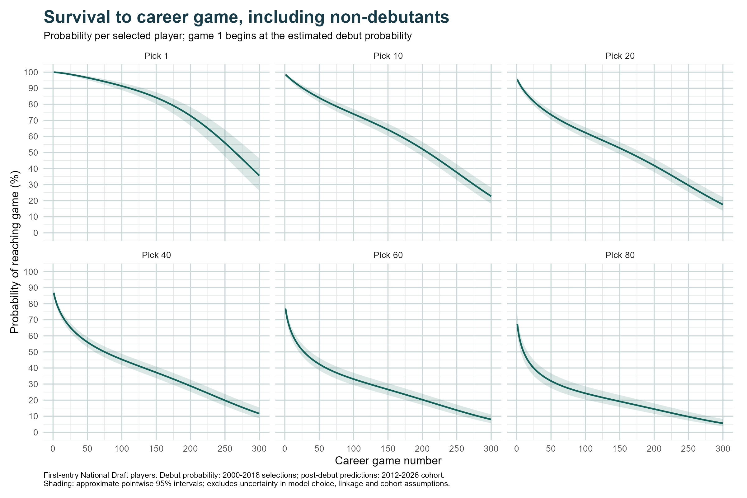
Figure 3. Estimated probability of reaching a given senior game for four selected picks. The accompanying survival data cover every pick from 1 to 104.
To obtain these probabilities we multiply the successive probabilities of continuing. For example, the probability of reaching game 100 is obtained by multiplying the probability of debuting by the 99 conditional probabilities of continuing after games 1 through 99.
4. Decomposing career points into match ratings and career length
A player’s total expected career rating points is the product of his expected career length and expected average rating points per game. The plot below shows how the two components vary, relatively speaking, with Pick number, and how their product also varies (as in the earlier plot).
Figure 4. Both ingredients start at 100. Their product, divided by 100, gives the career-value index.
We see, for example, that Pick 1 projects to 265.7 games at 10.85 points per game, and Pick 20 projects to 171 games at 9.37. Pick 20’s expected career length is therefore 64.4% of Pick 1’s, and its expected rating per game is 86.4% of Pick 1’s. Multiplying those percentages gives the 55.6% career value.
In the table below we estimate the relative effects of the differences in the various components of expected value, splitting the contribution from career length into the probability of debuting and then the expected career length assuming debuting occurred.
Table 3. Expected career length, rating per game and contributions to the value gap.
The numbers in this table are derived using a standard decomposition of a product method, an example of which is provided below:
We can repeat this analysis for all Pick numbers are see how the decomposition varies by Pick.
We see that, as Pick number increases the relative contribution of expected career length soon grows to become the major cause of the lower expected career rating points.
SUMMARY AND CONCLUSION
The main results from the analyses here are that:
If we use realised AFL Player Ratings as the measure of a player’s value across a career, the relative values of National Draft picks differ significantly from those in the original and the new AFL DVIs in that they fall away less quickly at higher Picks and stay relatively higher for later picks
A player’s expected career Rating Point tally depends significantly on the positions he plays but, once we adjust for this, the relative expected totals for a given Pick number are roughly the same for all positions. This might be used to argue for DVIs that differ by expected position, but implementing that would be impractical
Debut probabilities, expected career lengths, and expect Rating points for a given career game number all tend to decline with Pick number
If a player’s expected career Rating points tally is formed by multiplying his probability of debuting by his expected career length given that he debuts by his expected average Rating per game, a decomposition shows that the largest contributor to expected career Rating points is the player’s expected career length, especially for players who are drafted with high Pick numbers