The Real Mathematics of Winning Combination
/Back in late 2024 I wrote a blog post because I had recently started watching repeats of a British game show called Winning Combination that aired in 2020 and 2021 and in which nine contestants, numbered 1 to 9, answer questions in an attempt to become a part of a “final combination”.
That combination is simply the four numbers associated with the successful contestants and becomes the prize pool to be divided evenly amongst them if they complete a final challenge.
The elements of the game relevant to the analyses I performed then and will be correcting today are:
Winning contestants are determined one at a time, and each is allowed to place themselves in any of the remaining untaken positions in the combination. So, for example, if the player associated with the number 7 is first through, he or she can decide to place themselves in the thousands, hundreds, tens, or units position.
Because the prize pool is determined by the combination, contestants associated with larger numbers will prefer to place themselves further left in the combination, while those with smaller numbers will prefer to place themselves further right.
Once the combination has been set, contestants need to answer as many questions correctly as the number they are associated with. So, for example, our contestant numbered 7 would need to answer seven questions correctly to complete his or her part of the final task.
Questioning starts with the person in the units position and a time bank of 30 seconds. Time ticks down as the questions are being asked and the answer provided, and 5 seconds is added back to the clock for each correct answer provided (although the time bank is never allowed to go above 30 seconds). If the time bank reaches zero before the required number of correct answers have been provided, the game is over, and all four players receive nothing.
Questioning continues with the person in the tens, hundreds, and then thousands position.
If the contestant in the thousands position answers the requisite number of questions without the clock reaching zero, all four members of the combination share equally in the prize pool.
The five contestants who are not part of the final combination all receive nothing, regardless of the success or otherwise of the chosen four.
THE QUESTIONS
There are two interesting questions we can ask about the game:
Given a combination with none or some of the positions filled, where is the best place for the next contestant to place themselves? For example, if there are no positions filled and the contestant with number 5 wins through, in which position should he or she place themselves?
Once the combination has been determined, how likely is it that a team of a certain ability, defined by its ability to get questions right, will take home the prize?
OPTIMAL PLACEMENT
For this analysis we’re going to assume that:
All contestants, whatever their number, are equally talented, so any of them is as likely as any other to be the next one in the combination
The goal is to maximise the size of the final prize pool
When I ran this analysis in 2024 I ran 1 million simulations of the game and made the assumption that you could take a given state (say 6 in the thousands position with a 5 to place) and determine the best play by looking at all the simulated games that faced that position and compare the final value obtained when the 5 was placed in the hundreds, tens, or units crucially assuming that players placed themselves at random thereafter.
That last implicit assumption, which escaped me at the time, meant that I was optimising in a very narrow sense and not assuming that the players coming after would also make optimal placement decisions.
We now live in a world with LLMs that can code far better than I ever have or will, and that pick up on these subtleties, and so, with the help of Codex I have created a program that correctly identifies the optimal strategy for placing people at the game progresses.
That strategy, it turns out, is quite complex, but can be broken down into some high level heuristics that we can progressively add more details to in a structured way until we reveal the full optimal strategy.
The table at right reveals that the optimal strategy, on average, produces a final value of just under 8,109.
It also reveals a very simple set of heuristics for acheiving results close to the optimum without having to learn the optimum for every possible situation.
It tells us that, for example:
if the first contestant carries any of the numbers 1, 2, or 3, he or she should place themselves in the “lowest empty place”, which at that time of the game is the units
if, instead, the first contestant carries either a 4 or a 5, he or she should place themselves in the “empty-place rank 2 of 4”, which at that time of the game is the tens
contestants with a 6 should move into the hundreds position, and those with 7, 8, or 9 whould move into the thousands
the remaining rules should be interpreted in the same way with the term “lowest” meaning the category nearest the units
These suggestions seem sensible and show that the tricky decisions tend to come for the players with 4, 5 or 6.
Interestingly, this strategy has an expected value of 8,105.5 or about 99.96% of optimum. For practial purposes it is “optimal”.
We can though, as noted, identify the situations where the choice is more nuanced and define some rules to better capture these.
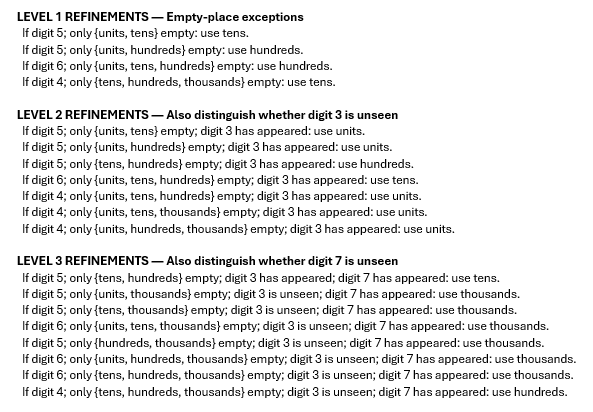
For example, in the Level 1 Refinements section at left we identify exceptions relating to the placement of 4s, 5s and 6s depending on which places remain vacant.
Level 2 Refinements then provide some additional adjustments depending on whether or not the person carrying 3 has already been placed.
Level 3 Refinements then do the same for the person carryng 7.
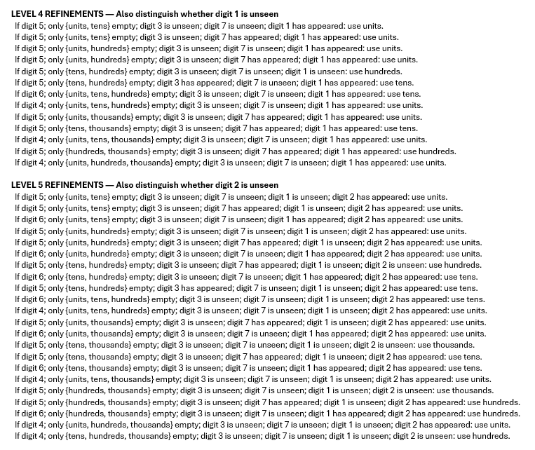
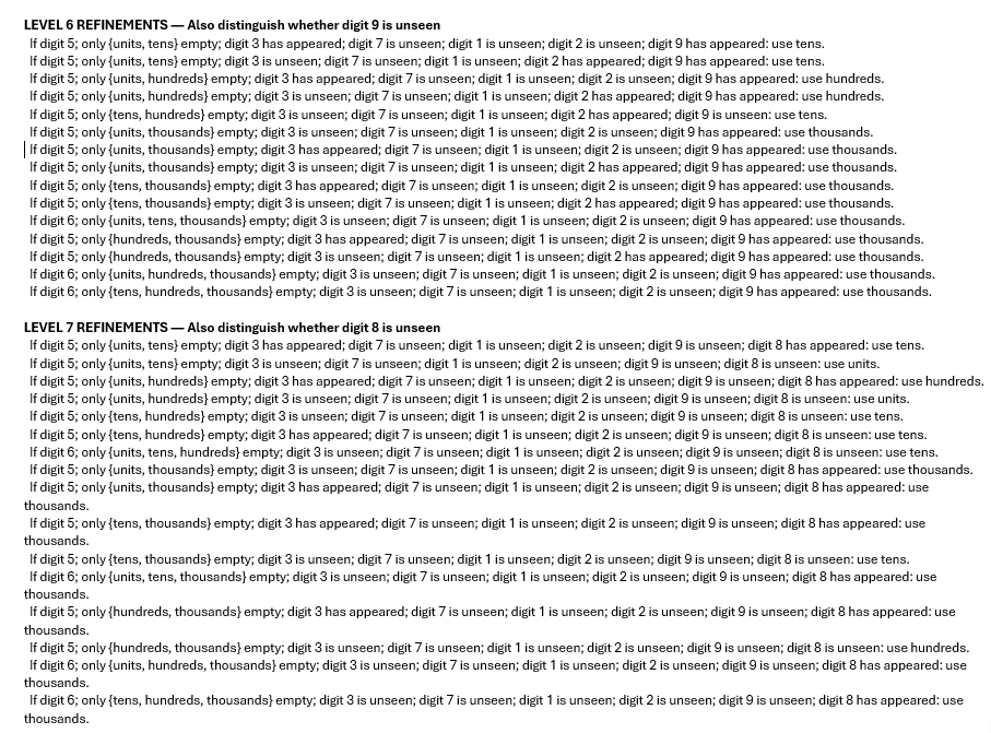
We can continue down this path and create Level 4 to Level 7 Refinements at which point we have a strategy that is the optimal one. Those other levels are provided in the images below (which can be clicked on to access larger versions), purely for completeness’ sake.
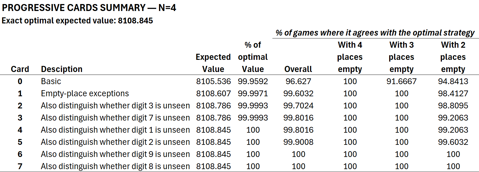
Whilst it would no doubt be possible to memorise all of these exceptions, the table at right reveals just how unnecessary this is.
As we’ve already noted, the expected value using just the initial, basic heuristic gets us 99.96% of the optimum. Adding only the empty-place exceptions for digits 4, 5 and 6 gets us to 99.997% of the optimum.
After that, it’s much more effort for practically zero return.
CHANCES OF VICTORY
In the earlier blog we also looked at the second question above. We’ll repeat that analysis here.
For this analysis we’re going to add a few more assumptions
All four contestants who form part of the final combination have the same, fixed probability of getting a question correct. This probability remains constant regardless of the time remaining in the time bank
When a question is answered correctly, the net effect on the time bank (relative to when the question started to be asked) is 0 seconds 50% of the time, and an addition of 1 second 50% of the time
When a question is answered incorrectly, the net effect on the time bank (relative to when the question started to be asked) is to subtract 4 seconds one-third of the time, 5 seconds one-third of the time, and 6 seconds one-third of the time
Very roughly speaking, this means that a final combination can get no more than six questions incorrrect between them before running out of time.
We’ll look at how the probability of victory varies as we change two things:
The final combination
The fixed probability of answering a question correctly (which we’ll vary between 35% and 75%)
The R code to perform this analysis also appears below and allows us to select a combination at random and then simulate the final question-asking process 10,000 times for that combination to calculate the proportion of the times that the contestants with that combination win or lose. It does this for 1m randomly-chosen combinations. (Since there are only 9x8x7x6 or 3,024 combinations, each will appear a number of times in the simulation).
Inspecting the outputs reveals that the order in which numbers appear in the final combination is irrelevant - so, for example, 9621 wins as often as 1269 - and what matters is the total of the numbers in the combination.
The chart below shows how the victory probability alters as we change that total and the probability of answering a question (click on it to access a larger version).
This tells us that, for example, given the assumptions we’ve made, a team with a final combination that adds to 20 (which is the average) needs to answer correctly about 72 or 73% of the time in order to be 50:50 chances of taking home the money.
One interesting aspect that this chart reveals is the high rate of payoff for improvements in question-answering ability from about 65% onwards. For example, with a combination total of 20, moving from a 65% rate for question-answering to a 70% rate lifts a team’s victory chances from 22% to 40%.
CODE FOR VICTORY CHANCES
library(ggplot2)
library(scales)
library(viridis)
library(grid)

calculate_state <- function(target, prob_right, init_time = 30L) {
    max_time <- 30L

    # win_prob[time + 1, remaining target + 1]
    win_prob <- matrix(
        0,
        nrow = max_time + 1L,
        ncol = target + 1L
    )

    # Unconditional expected seconds multiplied by the win indicator.
    win_seconds <- matrix(
        0,
        nrow = max_time + 1L,
        ncol = target + 1L
    )

    # If no answers remain, the game has been won.
    for (time_left in 1:max_time) {
        win_prob[time_left + 1L, 1L] <- 1
        win_seconds[time_left + 1L, 1L] <- time_left
    }

    p_correct_transition <- prob_right / 2
    p_wrong_transition <- (1 - prob_right) / 3

    for (remaining in 1:target) {
        target_col <- remaining + 1L
        previous_target_col <- remaining

        # Ascending order is important: incorrect-answer transitions
        # refer to lower time values in the current column.
        for (time_left in 1:max_time) {
            time_row <- time_left + 1L
            increased_time <- min(time_left + 1L, max_time)

            # Correct answer: right_time is 0 or 1.
            probability <- p_correct_transition * (
                win_prob[time_row, previous_target_col] +
                win_prob[increased_time + 1L, previous_target_col]
            )

            expected_seconds <- p_correct_transition * (
                win_seconds[time_row, previous_target_col] +
                win_seconds[increased_time + 1L, previous_target_col]
            )

            # Incorrect answer: wrong_time is 4, 5, or 6.
            for (penalty in 4:6) {
                new_time <- time_left - penalty

                if (new_time > 0) {
                    probability <- probability +
                        p_wrong_transition *
                        win_prob[new_time + 1L, target_col]

                    expected_seconds <- expected_seconds +
                        p_wrong_transition *
                        win_seconds[new_time + 1L, target_col]
                }
            }

            win_prob[time_row, target_col] <- probability
            win_seconds[time_row, target_col] <- expected_seconds
        }
    }

    p_win <- win_prob[init_time + 1L, target + 1L]
    unconditional_seconds <-
        win_seconds[init_time + 1L, target + 1L]

    mean_seconds_when_win <- if (p_win > 0) {
        unconditional_seconds / p_win
    } else {
        NA_real_
    }

    data.frame(
        ComboSum = target,
        ProbRight = prob_right,
        ProbWin = p_win,
        MeanSecsLeftWhenWin = mean_seconds_when_win
    )
}

parameter_grid <- expand.grid(
    ComboSum = 10:30,
    ProbRight = seq(0.35, 0.75, by = 0.01)
)

t0 <- Sys.time()

results_list <- Map(
    calculate_state,
    target = parameter_grid$ComboSum,
    prob_right = parameter_grid$ProbRight
)

game_results <- do.call(rbind, results_list)

game_results <- game_results[
    order(game_results$ProbWin, decreasing = TRUE),
]

write.csv(
    game_results,
    "ResultsBySumExact.csv",
    row.names = FALSE
)

print(Sys.time() - t0)

#################################

game_summary = game_results %>% group_by(ComboSum, ProbRight)

game_summary$Label = paste(round(game_summary$ProbWin*100,0),"%", sep = "")
game_summary$TextCol = ifelse(game_summary$ProbWin < 0.6, "A", "B")


plot_font <- "Source Sans 3"

p4 <- ggplot(
    game_summary,
    aes(x = ProbRight, y = ComboSum)
  ) +
  geom_tile(aes(fill = ProbWin)) +
  geom_text(
    aes(label = Label, colour = TextCol),
    family = plot_font,
    size = 3.8
  ) +
  scale_fill_viridis(
    name = "Estimated Win Prob",
    labels = label_percent()
  ) +
  scale_colour_manual(
    values = c("white", "grey25"),
    guide = "none"
  ) +
  scale_x_continuous(
    "Probability of answering correctly",
    labels = label_percent(),
    limits = c(0.34, 0.76),
    expand = expansion(mult = 0)
  ) +
  scale_y_continuous(
    "Combination total",
    expand = expansion(mult = 0)
  ) +
  labs(
    title = "Estimated Win Probability",
    subtitle = paste(
      "Right answers add 0 or 1 second;",
      "wrong answers subtract 4, 5, or 6 seconds"
    )
  ) +
  theme_minimal(
    base_family = plot_font,
    base_size = 12
  ) +
  theme(
    axis.title = element_text(
      face = "bold",
      colour = "#990000",
      size = 20
    ),
    axis.text = element_text(size = 12),

    plot.title = element_text(
      face = "bold",
      size = 30,
      margin = margin(b = 6)
    ),
    plot.subtitle = element_text(
      size = 18,
      colour = "grey30",
      margin = margin(b = 14)
    ),

    panel.border = element_rect(
      colour = "black",
      fill = NA,
      linewidth = 0.7
    ),
    panel.grid = element_blank(),

    legend.position = "none",
    plot.title.position = "plot"
  )

p4

ggsave(
  "win-probability.png",
  p4,
  width = 12,
  height = 8,
  dpi = 300,
  device = ragg::agg_png
)