Game Statistics and Game Outcomes
/My first Matter of Stats blog looked at how game statistics, averaged across an entire season for each team, are predictive of key season outcomes like ladder position, competition points and MARS Ratings.
This post summarises similar analyses, but here performed on a per-game basis, to answer the following questions:
- Are any of the game statistics for a single game predictive of its outcome (in terms of which team wins or by how much)?
- Which statistics are most predictive and which are least predictive?
- In particular, how predictive of game outcomes are the AFL Dream Team Points (we know they're not especially predictive of teams' season outcomes)?
Selecting the Best Game Statistics
In modeling team outcomes for full seasons we used only each team’s own game play statistics as inputs. In doing this and not controlling for the differences in each team's "strength of schedule" (ie the quality of the teams they faced during the season), there was an implicit assumption that each team faced, on average, an “average opposition”.
However, now that we're performing the analysis at the level of a single game, we need to use the game statistics of both the home and the away teams in each contest; it's the relative performance that matters.
There are some other, more minor changes. Several game statistics are removedbecause they relate directly to scoring, or virtually do so. Specifically, we exclude:
- The goals and behinds statistics because they directly define the score
- AFL Dream Team Points because they include goals and behinds (and a few other statistics)
- Goal Assists because they are highly correlated with goals
- Rebound 50s because inside 50s minus opponent rebound 50s is highly correlated with the number of goals scored (alas, because rebound 50s would otherwise be a powerful predictor)
- With some hesitation, centre clearances because the total number reflects the total number of goals scored in the game. The hesitation in excluding this statistic is because each team’s share of centre clearances is not perfectly correlated with goal-scoring, but winning the restarts certainly is a major step towards goal-scoring.
Additionally the following statistics are dropped to avoid collinearity in the models:
- Total Clearances (the sum of centre clearances and stoppage clearances)
- Total possessions (the sum of contested and uncontested possessions)
- Disposals (the sum of kicks and handballs)
- Frees Against (because the difference in the two teams' Frees For is the negative of the difference in their Frees Against)
So, here are the 18 remaining statistics, listed alphabetically:
- bounces, clangers, contested marks, contested possessions, disposal efficiency, frees for, goal accuracy, handballs, hit outs, inside 50s, kicks, marks, marks inside50, one-percenters, stoppage clearances, tackles, uncontested possessions.
Paired Statistics
Game statistics are available from 2001 onwards. I’ll focus on complete seasons so the games from the first half of 2013 are excluded. That leaves 2,254 games to model from the regular- and the post-season. (There’s missing data for 7 games in the period.)
I found, as did Tony, that the difference in team metrics was most often useful in modelling (for example, we need to include both the home team's inside 50s and the away team's inside 50s). Accordingly, I incorporate game statistics in pairs.
However, in a slight deviation from his work, the models I've built allow different coefficients for the home and the away teams for the same metric because this approach revealed some interesting differences between home and away team outcomes for particular game statistics.
Before I discuss those modelling results, however, let's first take a look at the correlation between the differences in the 18 game statistics I'm using and the game margin for all games over the 2001 to 2012 seasons.
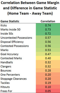
This table shows, for example, that there is a +0.74 correlation between the excess in the number of kicks registered for the home team relative to the away team, and the final game margin. Put another way, almost 50% of the variability in game margins can be explained by the difference in the number of kicks registered by the two teams in a game.
There are some interesting differences in this table when you compare it with the equivalent table from the previous blog in which we were correlating various season outcomes with these same statistics.
Kicks rise to the top of the table here (from 5th position with a correlation of only +0.36 with end of season ladder position). What this suggests is that having more kicks than your opponent in a single game is relatively important in determining that game's outcome, but that simply having more kicks in general is not especially predictive of a team's performance across a whole season.
Other entries from this table that are more in line with the equivalent table for season outcomes are those for marks inside 50 and inside 50s, which, when we looked at season outcomes, were less correlated only than the total goals scored per game metric. The correlations here are higher than the equivalent correlations in the previous blog (though of course the statistics are being used here to explain a different pool of variability).
All up, more of the differenced game statistics are highly correlated with game outcome than they were when expressed as season averages and correlated with season outcomes (ie 7 of the correlations here are above +0.50 compared with only 3 from the equivalent table in the previous blog, excluding goals).
The “All In” Model
With most of the game statistics looking useful let’s throw them all into a linear model of the score difference. We have over 2,000 games so we've plenty of degrees of freedom.
The table is ordered by the absolute value of the coefficient for the home team. Away team coefficients are negated to make them more readily comparable with the home team equivalent.

The table shows, for example, that each mark inside 50 for the home team adds 1.4 points to its expected margin of victory, and each mark inside 50 prevented by the home team adds 1.5 points to its expected victory margin.
The model intercept implies that the home team starts each game with a notional 27 point advantage (compared with the average home team score advantage of 8.7 over the period). The existence of a home team advantage is consistent with Tony’s findings, but the figure here is bigger than prior MAFL modeling. Note though that the coefficients for the home team are, in a majority of cases, smaller than the equivalent coefficients for the away team, so the expected victory margin for a home team that records game statistics numerically identical to those of its opponent, will be less than 27 points.
Nearly all the game statistics make a statistically significant contribution (p < 0.001) with the bottom few being the only exceptions. My view is that this is more because of the large data set than predictive importance.
Let me pause now to let the aficionados discuss… (I’m not one).
Did you notice the negative coefficients on frees-for and marks? More are bad?!
The adjusted R-squared for the model is 88.4%. (If we had included goals and behinds the model would of course have been perfect.)
That’s an adjusted correlation of +0.94, which is compelling.
The graph of fitted versus actual game margin bears out the model's goodness of fit. As well, a plot of the residuals suggests that they are very close to normally distributed so linear models are suited to this modeling task.

Home vs Away
Earlier I noted that I'd be allowing separate coefficients for the away team and home team versions of each game statistic. Why did I do this?
The right column in the table above shows the ratio of the away team and home team coefficients. If it is above 1.0 then the away team gets more impact from the game statistic than does the home team (moreso for those statistics towards the top of the table). Conversely, ratios below 1.0 imply a greater impact for the home team than the away team on this statistic. (Except for negative coefficients where the opposite is true.)
For example, the home team benefits relatively more from improvements in goal accuracy - about 3.2% more, which is only a marginal difference.
However, each kick has about 16% more benefit to the away team than the home team and, being at position 5 in importance, this difference could be impactful on the game outcomes.
The highest ratio for the away team is for tackles (4.7-to-1) but, being low down on the list, the absolute benefit is low.
Best-5 Model
The All In Model uses up 37 degrees of freedom, with coefficients for the 18 game statistics for the home and the away teams plus the intercept. Can we create a more parsimonious model that uses fewer game statistics – say 5 of them?

A first attempt includes the 5 variables from the All In model which had the largest absolute coefficients for the home team: marks inside 50, goal accuracy, inside 50s, clangers and frees for. It explains 82.6% of variance (ie a correlation of +0.91). But inspection of the coefficients suggested that the frees for variable wasn’t contributing much.
Instead, I constructed a Best-5 model using an iterative approach, adding one game statistic at a time (in pairs, one for the home team and the equivalent statistic for the away team) based on which of the remaining statistics provided the greatest improvement in adjusted R-squared. The table below shows the coefficients obtained and the order in which the variables were selected.
The Best-5 model explains 85.8% of variance (a correlation of +0.93) which is only a modest drop from the All In model (88.4% / +0.94) despite having less than one-third the number of variables.
Note also that:
- the intercept is smaller,
- marks are selected as the most predictive variable,
- otherwise the variables are consistent with the All In Model.
(As an aside, I trialled Linear Discriminant Analysis too. It produced similar results, so I won't present the details here.)
Modelling Win-Loss
Sometimes all we're concerned about is whether a team wins or loses. Are linear models effective at fitting this way of expressing the game outcome rather than the score difference? As a simple path let’s use “Home – Away > 0” as a binary outcome. (This treats a draw as an away win.)
Here the All-In linear model is 90% accurate.

The Top-5 linear model is slightly less accurate at about 88%.

Details of the variables in the Top-5 model appear in the table below, including the improvement in model fit (measured by accuracy) as each game statistic is added to the model. So, for example, knowing the number of kicks registered by each team in a game is enough to predict almost 80% of game outcomes from 2001 to 2012 (and, looking at the coefficients, we find that more kicks implies a higher probability of victory, and that there is only a very slight advantage for the home team of about 2.5%).

Dream Team Redux
My previous post explored the AFL’s Dream Team Point heuristic.
Dream Team Points = 6 x goals + behinds + 3 x kicks + 2 x handballs + 3 x marks + 4 x tackles + hitouts + frees for - 3 x frees against
If we select the winner of each game based on which team registers more Dream Team Points we achieve only about 81% accuracy. That seems remarkably poor considering that this statistic includes the game score (6 x goals + points)! The other base statistics it includes actually cause it to lose information!!!
Commentary
Do game-by-game findings match the season analysis? Not exactly.
- Marks inside 50 and inside 50s make the top-3 on both a game-by-game and season outcome basis
- Kicks, marks and goal accuracy were also-rans on the seasonal analysis but make the top-5 on the game-by-game basis
- The seasonal analysis allowed the use of rebound 50s and they made the top-3 for the Pretty Good Model (the model that matched the Dream Team statistic without using goals or behinds). So this is not an apples-for-apples comparison
As noted earlier I suspect that the between-game variability is significant, meaning that beating your opposition on the day is more important than achieving higher statistics across the season.
Would a coach care? I doubt it. (What stats do they look at on those computers in the coaching box or is it Twitter?) Telling players to take more marks, record more inside 50s etc doesn’t seem wholly constructive, at least for the pros.
If I’m generous, it might be useful to de-emphasise some of the game statistics that aren’t related to victory. For example, the tackle count seem consistently unimportant in game and season analysis. Although, I suspect the reason for this is that some tackles are far more important than others (e.g. in the defensive 50) but the data doesn’t differentiate these.
Should pundits care? Perhaps. They also have the benefit of 20-20 hindsight when analysing a game. But are they prepared to put aside their non-linear wisdom?
What about the many other factors that Tony has already shown to be meaningful? Some of the useful statistics that I recall from MAFL include venue experience and crowd size amongst many others. Ideally, these could be incorporated. That might became part of pre-game prediction of outcomes using historical game play statistics which brings me to…
Is any of this useful for betting? Not directly. The statistics used here are only available after the game and that’s too late for a bet.
However, the unsurprising finding that key statistics are very predictive of game outcomes (if not necessarily causal) means there is potentially useful information in them. The key now is to look at condensing past play into measures that improve the models.
As Tony’s recent blog has shown, an historical summary of some of the game statistics of a team does complement the bookie odds and so may improve the MAFL models.
Also, my last post found that the historical game statistics are reasonable predictors of the MARS Ratings which we know are very effective in the betting context.
Are teams different? The models are all generalized for both the home and away team. That potentially loses valuable information. To the point above, perhaps Sydney and Hawthorn are better at kicks that count; or well-timed tackles. Maybe, there are weaknesses in the defensive structures of GWS and Melbourne.
There’s many a post to be written about whether different teams have clearly differentiable styles, whether those styles point to different winning strategies, and how those strength differences play out.
Tony has encouraged me particularly to look at the Offensive Defensive Model (ODM) which is a path to exploring these matters.
Are the game statistics consistent over seasons? The last blog showed some drift in the statistics over the period 2001 to 2012. As a teaser, there’s some interesting trends that I’d like to return to in a future post.
What about player statistics? All the game statistics are available on a player-by-player basis. It would be interesting to see whether there’s a way to determine player impact or play value. I would certainly expect to beat the AFL Dream Team Points that are prominently published for players.
Having clearly demonstrated the limitations of the post’s own analysis it is time to sign off.