Can We Do Better Than The Binary Logit?

To say that there's a 'bit in this blog' is like declaring the 100 year war 'a bit of a skirmish'.

I'll start by broadly explaining what I've done. In a previous blog I constructed 12 models, each attempting to predict the winner of an AFL game. The 12 models varied in two ways, firstly in terms of how the winning team was described:

• Model 1 type models sought to estimate the probability of the higher-ranked MARS team winning
• Model 2 type models sought to estimate the probability of the home team winning, and
• Model 3 type models sought to estimate the probability of the favourite team winning

We created 4 versions of each of these model types by selecting different sets of variables with which to explain the relevant probability. These variables variously described the teams' MARS Ratings, bookie prices and home team status.

All 12 models were fitted to the results for seasons 2006 to 2009 and then applied to season 2010 for which, among other things, the profitability of each model was calculated assuming that a Kelly betting strategy was applied to each model's probability estimates for that season.

Of the 12 models, 5 of them would have been profitable in 2010, most notably model 3d, which produced a 17.7% ROI.

Throughout that blog, the modelling algorithm I used was the binary logit, which is just one of a large number of statistical algorithms that can be applied to the task of producing probability estimates. In this blog, I've looked at a few more such algorithms - well 42 more of them actually.

Armed with this statistical battery, I've broadly replicated and expanded the analysis from the previous blog.

I've also modified it a little. In the previous blog, for example, I allowed myself the luxury of identifying the best performing model variation post hoc, by estimating the 2010 ROI for all 12 model variations. Were I back at the start of season 2010, absent a time-travelling accident that's yet to have happened, this strategy would not have been available to me. More logically, I'd have opted for the model variation with the highest ROI for the 2006-2009 period, which in the binary logit case would have been Model variant 2d, which produced a 9.2% ROI across 2007-2009 and a more modest 1.3% ROI for 2010. Still a profit, but not quite as big a profit.

For this blog I've used this more realistic method to assess the forecast performance of each statistical modelling approach.

Before I show you the data from this exercise there's just one other thing to note. Some of the statistical modelling approaches that I've used - unlike the binary logit - have what are called 'tuning parameters', with which the user can alter the details of the data fitting process. For these algorithms I needed to select a best set of values for all the tuning parameters, which I did by using the caret package default of maximising the accuracy of the fitted models over the fitting period (ie 2006-2009). A model's prediction is considered to be accurate (ie correct) if it assigns a probability of greater than 50% to the winning team. (As in the previous blog, draws have been excluded from the analysis).

Statistical algorithms that have been tuned in this way carry the designation '(T)' in the table below. Those carrying the designation '(U)' are for algorithms that are tunable but for which I used only the default tuning parameters, and those carrying neither a '(T)' nor a '(U)' are non-tunable algorithms, such as the binary logit.

(click on the chart for a larger version).

The numbers to focus on first - the "takeaway" numbers to borrow from the business lexicon - are those in the penultimate column. These provide the ROI that would have been achieved by Kelly wagering on the relevant statistical model's probability forecasts for 2010.

So, for example, if you'd opted for the Flexible Discriminant Analysis algorithm, tuned it for all 12 model variants to maximise the accuracy over the 2006-2009 period for each variant, then selected the model variant for which this approach would have yielded the highest ROI across 2006-2009 - the 3d variant in this case - then you'd have enjoyed a whopping 38.8% ROI in 2010. Sweet ... though regretably only in hindsight.

Following this same approach, 20 other statistical modelling algorithms would also have returned a positive ROI for 2010, ranging from a 21.7% ROI for Stepwise Linear Discriminant Analysis to just 0.4% for a Support Vector Machine with a Polynomial Kernel. (If you want to know more about any of the cavalcade of statistical modelling algorithms that I've used in this blog, I refer you to the R website and, especially, to the very fine caret package, without which the calculations needed for this blog would never have been attempted.)

For a while that was where I thought I'd finish this blog. I'd identified a few promising potential modelling approaches for 2011 and I now knew how to use the caret package. Then I discovered that the caret package allowed me to define my own performance metric, so rather than tuning each statistical algorithm to maximise its accuracy across the 2006-2009 period, I could instead tune it to maximise its ROI for that period. This seemed to me to be a method likely to produce higher ROIs.

It takes a while - near enough a day - to fit just 1 model variation to all 42 models using this approach, and I couldn't justify the (read: another) 12 days of effort that would be necessary to fit all 12 variations. Instead, I chose just 3 variations, the three that appeared most often as the best variant in the earlier analysis amongst those statistical modelling algorithms that produced a positive ROI for 2006-2009. These variants were 2d, 3c, and 3d.

The next step in the analysis was then to fit these three variants for all 42 statistical algorithms, this time tuning to maximise the ROI for 2006-2009 and then applying this optimised model to season 2010.

Here are the results (click on the chart for a larger version):

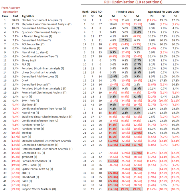
The money numbers here are those under the "Fitted to 2010" section. These are the ROIs of each model optimised for ROI across 2006-2009 and then applied to 2010. Figures that appear against a grey background are ROIs that are higher with this more direct ROI-based optimisation approach than the equivalent ROI obtained in the earlier table using the more indirect accuracy-based optimisation approach.

So, for example, the Generalised Additive Spline algorithm produced a 16.2% ROI for 2010 here, which is shown on a grey background because it exceeds the 10.6% ROI that we produced using this statistical algorithm in the previous table.

The general message from this chart is that optimising for ROI produces superior 2010 returns for about one half of the algortihms if we use variant 2d (and much less than one-half of the profitable algorithms), for only a handful of algorithms if we use variant 3c, and for slightly less than one-half of the algorithms if we use variant 3d. Most importantly, however, all but 4 of the profitable algorithms are more profitable under this new optimisation approach if we use variant 3d.

Under the previous optimisation approach, only 3 statistical algorithms produced double-digit returns in 2010; under the new optimisation approach with variant 3d, 8 statistical algorithms produce such returns.

How then to select the most promising algorithms to consider for season 2011?

The simplest way would be to choose the algorithm with the highest best-case 2010 ROI, which would catapult Flexible Discriminant Analysis and earth to the top of the pile. These algorithms probably do deserve a spot on the shortlist, but the fact that these same algorithms generated losses for one of the tested variants does make me a bit nervous about the replicability of their 2010 results.

Other algorithms such as Generalised Additive Spline, Quadratic Discriminant Analysis and Generalised Additive all have the appealling characteristic of making at least a modest profit for every tested variant. (The ROIs for some algorithms have a stochastic component because the optimum tuning parameters that are selected vary from run to run since they're based on the particular sample of the data that is selected for a run. The ROIs shown in the table are the average across 10 such runs for each algorithm. The Generalised Additive Spline model, though its mean ROI is positive for each variant, has a large standard deviation of that ROI for variant 3c. This makes that algorithm slightly less attractive.)

A final set of algorithms for consideration - Binary Logit, PLR (which stands for Penalised Linear Regression), Penalised Discriminant Analysis (1 and 2), Linear Discriminant Analysis, Generalised Additive Loess and Conditional Inference Tree Forest - all also produce positive ROIs for all three variants, though quite small ROIs for one or two variants.

I'll be looking more closely at the performance of these three sets of algorithms in a future blog and determining, for example, whether the ROI comes from a large or small numbers of wagers - the larger the number, the more confident we can feel that the ROI was not merely the result of a few 'lucky' wagers in 2010.

To finish on a slightly technical note, it's interesting, I think, to note the apparent overfitting of the PCA Neural Net, Conditional Inference Tree (tuned and untuned), Random Forest (tuned and untuned) and Treebag algorithms, as evidenced by their sterling performance in the fitting period and their poor performance post sample in 2010. You could also level this same criticism at the Conditional Inference Tree Forest algorithm, though to a somewhat lesser extent. The Tree and Forest methods are sometimes held out as being less susceptible to overfitting than other algorithms, though this is clearly not the case here. 

Anyway, enough for now.